equilibrium
Description of a 2D, axi-symmetric, tokamak equilibrium; result of an equilibrium code.
Maximum occurrences (MDS+ backend only): 3
New in version 3.1.0: lifecycle status active
Changed in version 4.2.0.
ids_propertiesstructure
See common IDS structure reference: ids_properties.
vacuum_toroidal_fieldstructure¶Characteristics of the vacuum toroidal field (used in rho_tor […]
Characteristics of the vacuum toroidal field (used in rho_tor definition and in the normalization of current densities)
vacuum_toroidal_field/r0 ⇹mFLT_0D¶Reference major radius where the vacuum toroidal magnetic field […]
Reference major radius where the vacuum toroidal magnetic field is given (usually a fixed position such as the middle of the vessel at the equatorial midplane)
grids_ggd(itime)AoS¶Grids (using the Generic Grid Description), for various time […]
Grids (using the Generic Grid Description), for various time slices. The timebase of this array of structure must be a subset of the time_slice timebase
1 |
New in version 3.18.0: lifecycle status alpha
grids_ggd(itime)/grid(i1)AoS¶Set of GGD grids for describing the equilibrium, at a given time […]
Set of GGD grids for describing the equilibrium, at a given time slice
1 |
|
grids_ggd(itime)/grid(i1)/identifierstructure¶Grid identifier
Grid identifier
This is an identifier. See ggd_identifier for the available options.
grids_ggd(itime)/grid(i1)/pathSTR_0D¶Path of the grid, including the IDS name, in case of implicit […]
Path of the grid, including the IDS name, in case of implicit reference to a grid_ggd node described in another IDS. To be filled only if the grid is not described explicitly in this grid_ggd structure. Example syntax: #wall:2/description_ggd(1)/grid_ggd, means that the grid is located in the wall IDS, occurrence 2, with relative path description_ggd(1)/grid_ggd, using Fortran index convention (here : first index of the array)
grids_ggd(itime)/grid(i1)/space(i2)AoS¶Set of grid spaces
Set of grid spaces
Click here for further documentation.
1 |
|
grids_ggd(itime)/grid(i1)/space(i2)/identifierstructure¶Space identifier
Space identifier
This is an identifier. See ggd_space_identifier for the available options.
grids_ggd(itime)/grid(i1)/space(i2)/identifier/nameSTR_0D¶Short string identifier
Short string identifier
grids_ggd(itime)/grid(i1)/space(i2)/geometry_typestructure¶Type of space geometry (0: standard, 1:Fourier, >1: Fourier with […]
Type of space geometry (0: standard, 1:Fourier, >1: Fourier with periodicity)
grids_ggd(itime)/grid(i1)/space(i2)/geometry_type/nameSTR_0D¶Short string identifier
Short string identifier
grids_ggd(itime)/grid(i1)/space(i2)/coordinates_type(i3)AoS¶Type of coordinates describing the physical space, for every […]
Type of coordinates describing the physical space, for every coordinate of the space. The size of this node therefore defines the dimension of the space.
This is an identifier. See coordinate_identifier for the available options.
1 |
|
Changed in version 4.0.0: Type changed from INT_1D
grids_ggd(itime)/grid(i1)/space(i2)/coordinates_type(i3)/nameSTR_0D¶Short string identifier
Short string identifier
grids_ggd(itime)/grid(i1)/space(i2)/objects_per_dimension(i3)AoS¶Definition of the space objects for every dimension (from one […]
Definition of the space objects for every dimension (from one to the dimension of the highest-dimensional objects). The index correspond to 1=nodes, 2=edges, 3=faces, 4=cells/volumes, …. For every index, a collection of objects of that dimension is described.
1 |
|
grids_ggd(itime)/grid(i1)/space(i2)/objects_per_dimension(i3)/object(i4)AoS¶Set of objects for a given dimension
Set of objects for a given dimension
1 |
|
grids_ggd(itime)/grid(i1)/space(i2)/objects_per_dimension(i3)/object(i4)/boundary(i5)AoS¶Set of (n-1)-dimensional objects defining the boundary of this […]
Set of (n-1)-dimensional objects defining the boundary of this n-dimensional object
1 |
|
grids_ggd(itime)/grid(i1)/space(i2)/objects_per_dimension(i3)/object(i4)/boundary(i5)/indexINT_0D¶Index of this (n-1)-dimensional boundary object
Index of this (n-1)-dimensional boundary object
grids_ggd(itime)/grid(i1)/space(i2)/objects_per_dimension(i3)/object(i4)/boundary(i5)/neighbours(:)INT_1D¶List of indices of the n-dimensional objects adjacent to the […]
List of indices of the n-dimensional objects adjacent to the given n-dimensional object. An object can possibly have multiple neighbours on a boundary
1 |
|
grids_ggd(itime)/grid(i1)/space(i2)/objects_per_dimension(i3)/object(i4)/geometry(:)mixedFLT_1D¶Geometry data associated with the object, its detailed content […]
Geometry data associated with the object, its detailed content is defined by ../../geometry_content. Its dimension depends on the type of object, geometry and coordinate considered.
1 |
|
grids_ggd(itime)/grid(i1)/space(i2)/objects_per_dimension(i3)/object(i4)/nodes(:)INT_1D¶List of nodes forming this object (indices to objects_per_dimension(1)%object(:) […]
List of nodes forming this object (indices to objects_per_dimension(1)%object(:) in Fortran notation)
1 |
|
grids_ggd(itime)/grid(i1)/space(i2)/objects_per_dimension(i3)/object(i4)/measurem^dimensionFLT_0D¶Measure of the space object, i.e. […]
Measure of the space object, i.e. physical size (length for 1d, area for 2d, volume for 3d objects,…)
grids_ggd(itime)/grid(i1)/space(i2)/objects_per_dimension(i3)/object(i4)/geometry_2d(:,:)mixedFLT_2D¶2D geometry data associated with the object. […]
2D geometry data associated with the object. Its dimension depends on the type of object, geometry and coordinate considered. Typically, the first dimension represents the object coordinates, while the second dimension would represent the values of the various degrees of freedom of the finite element attached to the object.
1 |
|
2 |
|
New in version >3.35.0.
grids_ggd(itime)/grid(i1)/space(i2)/objects_per_dimension(i3)/geometry_contentstructure¶Content of the ../object/geometry node for this dimension
Content of the ../object/geometry node for this dimension
This is an identifier. See ggd_geometry_content_identifier for the available options.
New in version >3.33.0.
grids_ggd(itime)/grid(i1)/space(i2)/objects_per_dimension(i3)/geometry_content/nameSTR_0D¶Short string identifier
Short string identifier
grids_ggd(itime)/grid(i1)/grid_subset(i2)AoS¶Grid subsets
Grid subsets
1 |
|
grids_ggd(itime)/grid(i1)/grid_subset(i2)/identifierstructure¶Grid subset identifier
Grid subset identifier
Click here for further documentation.
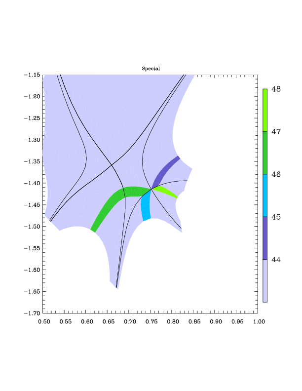
This is an identifier. See ggd_subset_identifier for the available options.
grids_ggd(itime)/grid(i1)/grid_subset(i2)/identifier/nameSTR_0D¶Short string identifier
Short string identifier
grids_ggd(itime)/grid(i1)/grid_subset(i2)/dimensionINT_0D¶Space dimension of the grid subset elements, using the convention […]
Space dimension of the grid subset elements, using the convention 1=nodes, 2=edges, 3=faces, 4=cells/volumes
grids_ggd(itime)/grid(i1)/grid_subset(i2)/element(i3)AoS¶Set of elements defining the grid subset. […]
Set of elements defining the grid subset. An element is defined by a combination of objects from potentially all spaces
1 |
|
grids_ggd(itime)/grid(i1)/grid_subset(i2)/element(i3)/object(i4)AoS¶Set of objects defining the element
Set of objects defining the element
1 |
|
grids_ggd(itime)/grid(i1)/grid_subset(i2)/element(i3)/object(i4)/spaceINT_0D¶Index of the space from which that object is taken
Index of the space from which that object is taken
grids_ggd(itime)/grid(i1)/grid_subset(i2)/base(i3)AoS¶Set of bases for the grid subset. […]
Set of bases for the grid subset. For each base, the structure describes the projection of the base vectors on the canonical frame of the grid.
1 |
|
grids_ggd(itime)/grid(i1)/grid_subset(i2)/base(i3)/jacobian(:) ⇹mixedFLT_1D¶Metric Jacobian
Metric Jacobian
1 |
grids_ggd(itime)/grid(i1)/grid_subset(i2)/base(i3)/tensor_covariant(:,:,:) ⇹mixedFLT_3D¶Covariant metric tensor, given on each element of the subgrid […]
Covariant metric tensor, given on each element of the subgrid (first dimension)
1 |
|
2 |
|
3 |
|
grids_ggd(itime)/grid(i1)/grid_subset(i2)/base(i3)/tensor_contravariant(:,:,:) ⇹mixedFLT_3D¶Contravariant metric tensor, given on each element of the subgrid […]
Contravariant metric tensor, given on each element of the subgrid (first dimension)
1 |
|
2 |
|
3 |
|
grids_ggd(itime)/grid(i1)/grid_subset(i2)/metricstructure¶Metric of the canonical frame onto Cartesian coordinates
Metric of the canonical frame onto Cartesian coordinates
grids_ggd(itime)/grid(i1)/grid_subset(i2)/metric/jacobian(:) ⇹mixedFLT_1D¶Metric Jacobian
Metric Jacobian
1 |
grids_ggd(itime)/grid(i1)/grid_subset(i2)/metric/tensor_covariant(:,:,:) ⇹mixedFLT_3D¶Covariant metric tensor, given on each element of the subgrid […]
Covariant metric tensor, given on each element of the subgrid (first dimension)
1 |
|
2 |
|
3 |
|
grids_ggd(itime)/grid(i1)/grid_subset(i2)/metric/tensor_contravariant(:,:,:) ⇹mixedFLT_3D¶Contravariant metric tensor, given on each element of the subgrid […]
Contravariant metric tensor, given on each element of the subgrid (first dimension)
1 |
|
2 |
|
3 |
|
time_slice(itime)AoS¶Set of equilibria at various time slices
Set of equilibria at various time slices
1 |
time_slice(itime)/boundarystructure¶Description of the plasma boundary. […]
Description of the plasma boundary. The boundary can be either the real separatrix (provided by a free boundary equilibrium solver) or the 0.99x psi_norm flux surface provided by a fixed boundary equilibrium
time_slice(itime)/boundary/outlinestructure¶RZ outline of the plasma boundary
RZ outline of the plasma boundary
time_slice(itime)/boundary/psi_norm ⇹1FLT_0D¶Value of the normalized poloidal flux at which the boundary is […]
Value of the normalized poloidal flux at which the boundary is taken, the flux being normalized to its value at the separatrix (so psi_norm = 1 if the boundary is the separatrix)
time_slice(itime)/boundary/psi ⇹WbFLT_0D¶Value of the poloidal flux at which the boundary is taken. […]
Value of the poloidal flux at which the boundary is taken. For a positive plasma current (counter-clockwise when viewed from above), increases from the magnetic axis to the boundary
time_slice(itime)/boundary/geometric_axisstructure¶RZ position of the geometric axis (defined as (Rmin+Rmax) / 2 […]
RZ position of the geometric axis (defined as (Rmin+Rmax) / 2 and (Zmin+Zmax) / 2 of the boundary)
time_slice(itime)/boundary/minor_radius ⇹mFLT_0D¶Minor radius of the plasma boundary (defined as (Rmax-Rmin) / […]
Minor radius of the plasma boundary (defined as (Rmax-Rmin) / 2 of the boundary)
time_slice(itime)/boundary/elongation ⇹1FLT_0D¶Elongation of the plasma boundary
Elongation of the plasma boundary
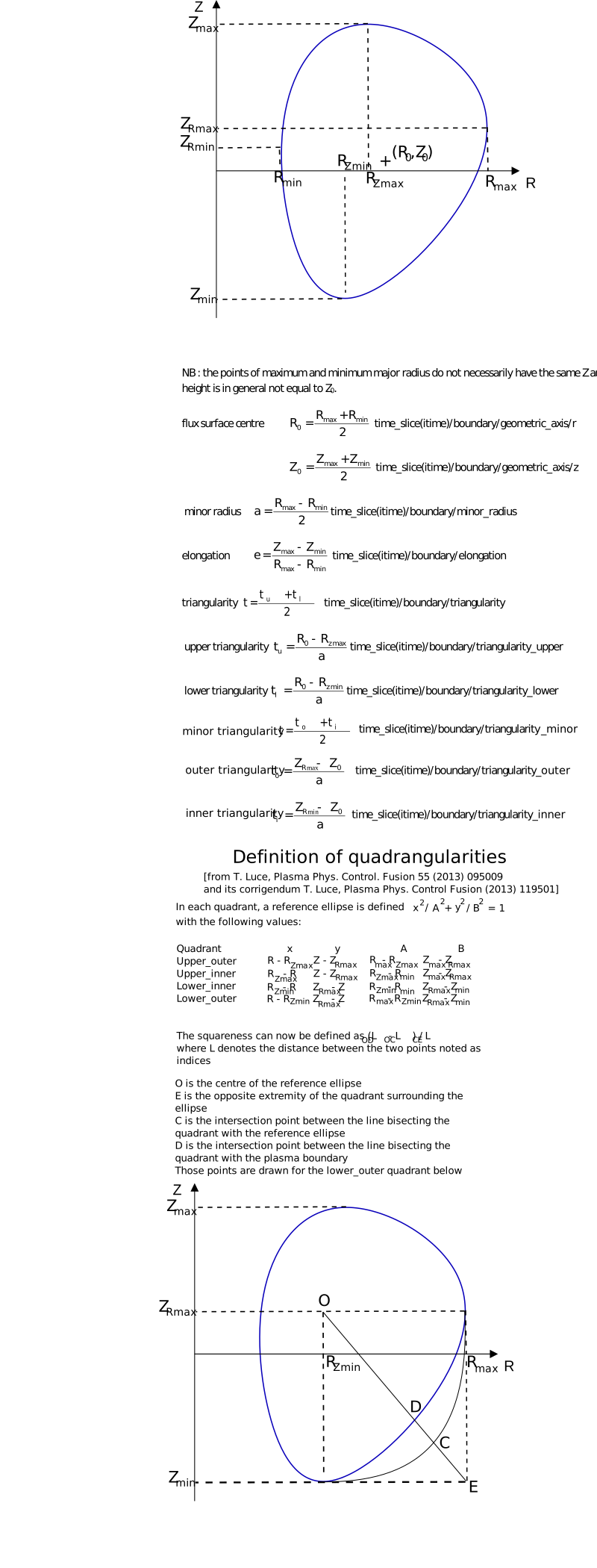
time_slice(itime)/boundary/triangularity ⇹1FLT_0D¶Triangularity of the plasma boundary
Triangularity of the plasma boundary
time_slice(itime)/boundary/triangularity_upper ⇹1FLT_0D¶Upper triangularity of the plasma boundary
Upper triangularity of the plasma boundary
time_slice(itime)/boundary/triangularity_lower ⇹1FLT_0D¶Lower triangularity of the plasma boundary
Lower triangularity of the plasma boundary
time_slice(itime)/boundary/squareness_upper_inner ⇹1FLT_0D¶Upper inner squareness of the plasma boundary (definition from […]
Upper inner squareness of the plasma boundary (definition from T. Luce, Plasma Phys. Control. Fusion 55 (2013) 095009)
New in version 3.18.0: lifecycle status alpha
time_slice(itime)/boundary/squareness_upper_outer ⇹1FLT_0D¶Upper outer squareness of the plasma boundary (definition from […]
Upper outer squareness of the plasma boundary (definition from T. Luce, Plasma Phys. Control. Fusion 55 (2013) 095009)
New in version 3.18.0: lifecycle status alpha
time_slice(itime)/boundary/squareness_lower_inner ⇹1FLT_0D¶Lower inner squareness of the plasma boundary (definition from […]
Lower inner squareness of the plasma boundary (definition from T. Luce, Plasma Phys. Control. Fusion 55 (2013) 095009)
New in version 3.18.0: lifecycle status alpha
time_slice(itime)/boundary/squareness_lower_outer ⇹1FLT_0D¶Lower outer squareness of the plasma boundary (definition from […]
Lower outer squareness of the plasma boundary (definition from T. Luce, Plasma Phys. Control. Fusion 55 (2013) 095009)
New in version 3.18.0: lifecycle status alpha
time_slice(itime)/boundary/closest_wall_pointstructure¶Position and distance to the plasma boundary of the point of […]
Position and distance to the plasma boundary of the point of the first wall which is the closest to plasma boundary
Changed in version 4.0.0: Renamed from ../boundary_separatrix/closest_wall_point
New in version >3.
time_slice(itime)/boundary/dr_dz_zero_pointstructure¶Outboard point on the separatrix on which dr/dz = 0 (local maximum […]
Outboard point on the separatrix on which dr/dz = 0 (local maximum of the major radius of the separatrix). In case of multiple local maxima, the closest one from z=z_magnetic_axis is chosen.
Changed in version 4.0.0: Renamed from ../boundary_separatrix/dr_dz_zero_point
New in version >3.
time_slice(itime)/boundary/gap(i1)AoS¶Set of gaps, defined by a reference point and a direction.
Set of gaps, defined by a reference point and a direction.
1 |
|
Changed in version 4.0.0: Renamed from ../boundary_separatrix/gap
New in version >3.
time_slice(itime)/boundary/gap(i1)/nameSTR_0D¶Short string identifier (unique for a given device)
Short string identifier (unique for a given device)
time_slice(itime)/boundary/gap(i1)/descriptionSTR_0D¶Description, e.g. […]
Description, e.g. mid-plane gap
New in version >3.
time_slice(itime)/boundary/gap(i1)/r ⇹mFLT_0D¶Major radius of the reference point
Major radius of the reference point
time_slice(itime)/boundary/gap(i1)/z ⇹mFLT_0D¶Height of the reference point
Height of the reference point
time_slice(itime)/boundary/rho_tor ⇹mFLT_0D¶Toroidal flux coordinate at the selected plasma boundary
Toroidal flux coordinate at the selected plasma boundary
Changed in version 4.1.0: Renamed from ../global_quantities/rho_tor_boundary
New in version >4.0.0.
time_slice(itime)/boundary/phi ⇹WbFLT_0D¶Toroidal flux at the selected plasma boundary. […]
Toroidal flux at the selected plasma boundary. Positive when the toroidal magnetic field is counter-clockwise when viewed from above
New in version >4.0.0.
time_slice(itime)/boundary/phi_poloidal_current ⇹WbFLT_0D¶Toroidal flux at the selected plasma boundary generated by the […]
Toroidal flux at the selected plasma boundary generated by the plasma poloidal current. Positive when the toroidal magnetic field is counter-clockwise when viewed from above
New in version >4.0.0.
time_slice(itime)/contour_treestructure¶Contour tree (Reeb graph) of the poloidal flux, encoding the […]
Contour tree (Reeb graph) of the poloidal flux, encoding the topological structure of the equilibrium through its critical points and limiter points. Nodes represent critical points of the poloidal flux (O-points, X-points) and limiter points where the plasma boundary touches the first wall. Edges connect nodes that are topologically adjacent in psi_norm space, meaning no other node lies between them. The tree captures the nesting structure of flux surfaces, the connectivity between plasma regions, the separatrix topology, and the locations of limiter contacts. Normalised poloidal flux, psi_norm = (psi - psi_axis) / (psi_boundary - psi_axis), defines all ordering conventions.
New in version 4.0.0: lifecycle status alpha
New in version >3.
time_slice(itime)/contour_tree/node(i1)AoS¶Set of critical points and limiter points of the poloidal flux. […]
Set of critical points and limiter points of the poloidal flux. Each node is defined by its critical type (see critical_type), node type (see node_type), and position within the poloidal plane. All ordering rules below are defined in terms of normalised poloidal flux, psi_norm = (psi - psi_axis) / (psi_boundary - psi_axis), which is 0 at the magnetic axis and 1 at the plasma boundary. Nodes are partitioned into two groups: critical points (critical_type 0, 1, 2) occupy the leading indices, followed by limiter points (critical_type 3). Within each partition, nodes are ordered by ascending psi_norm; ties are broken by ascending R, then ascending Z. Node 0 must contain the primary O-point (magnetic axis), which has psi_norm = 0. Node 1 must contain the primary X-point, defined as the X-point with the lowest psi_norm value. For double-null divertor (DND) configurations, the secondary X-point has a higher psi_norm value and must be stored at a higher node index than the primary; the two psi_norm values are always distinct in practice. For limiter-bounded plasmas where no X-point defines the LCFS, node 1 should contain the X-point with the lowest psi_norm value (nearest to the plasma boundary), if any X-point exists. If no X-points exist, nodes are ordered by ascending psi_norm starting from node 1. For doublet or multi-region plasmas, each confined plasma region has its own O-point; additional O-points follow the same ascending psi_norm ordering. When limiter points are absent, only the critical point partition is present and the ordering is unchanged from earlier versions. The node_type identifier distinguishes O-points that represent confined plasma regions (node_type = plasma) from vacuum field extrema (node_type = vacuum).
1 |
|
time_slice(itime)/contour_tree/node(i1)/critical_typeINT_0D¶Critical-point type of the poloidal flux: 0 = local minimum, […]
Critical-point type of the poloidal flux: 0 = local minimum, 1 = saddle (X-point), 2 = local maximum, 3 = limiter point. Whether the magnetic axis is a minimum or maximum of psi depends on the sign of the plasma current. A limiter point represents a point on the first wall where the plasma boundary makes contact. Limiter point nodes are inserted by splitting an existing tree edge at the limiter point’s psi level; they have degree 2 in the tree. A limiter point is valid only if it belongs to the same connected component as at least one O-point in the subgraph obtained by removing all saddle nodes (critical_type = 1). Limiter points store the last closed flux surface passing through the limiter point in their levelset
time_slice(itime)/contour_tree/node(i1)/node_typestructure¶Identifies whether this node represents a confined plasma feature […]
Identifies whether this node represents a confined plasma feature or a vacuum field feature. Only meaningful for O-point nodes (critical_type 0 or 2). Limiter points are always plasma features. X-points and saddle points do not require classification
This is an identifier. See equilibrium_contour_tree_node_type_identifier for the available options.
time_slice(itime)/contour_tree/node(i1)/node_type/nameSTR_0D¶Short string identifier
Short string identifier
time_slice(itime)/contour_tree/node(i1)/psi ⇹WbFLT_0D¶Value of the poloidal flux at the node location. […]
Value of the poloidal flux at the node location. Whether psi increases or decreases from the magnetic axis outward depends on the sign of the plasma current. All ordering rules in the contour tree (node ordering, levelset segment ordering) are defined in terms of normalised poloidal flux, psi_norm = (psi - psi_axis) / (psi_boundary - psi_axis), which always increases from 0 at the magnetic axis to 1 at the plasma boundary
time_slice(itime)/contour_tree/node(i1)/levelset(i2)AoS¶Poloidal flux contour segments at the node’s psi value that are […]
Poloidal flux contour segments at the node’s psi value that are topologically connected to the node. Each element of the array of structures stores one distinct contour segment. Only segments whose contour passes through the node are included; disconnected contours that share the same psi value but are spatially remote must be excluded. For O-points (flux extrema), no contour passes through the extremum and this field must contain a single entry with empty r and z arrays. For limiter points, the levelset contains the last closed flux surface (LCFS) that passes through the limiter point. For X-points, the segments are ordered as follows: segment 0 is the last closed flux surface (LCFS), the closed contour bounding the confined plasma that passes through the X-point. Segments 1..N are divertor or scrape-off layer leg contours, ordered by their departure angle from the X-point measured counterclockwise from the outboard midplane (theta=0 at R_max, Z of the X-point) in the standard (R, Z) poloidal plane. A standard single-null divertor (SND) X-point has 2 segments: the LCFS and the divertor legs. A double-null divertor (DND) has 2 segments per X-point; the primary X-point (lower psi_norm, closer to the magnetic axis) is stored at a lower node index than the secondary, so their levelsets are unambiguously associated. An exact snowflake, where two X-points merge into a single higher-order null with 6 separatrix branches, produces 3 segments: the LCFS and 2 distinct divertor channel contours.
1 |
|
time_slice(itime)/contour_tree/node(i1)/levelset(i2)/r(:) ⇹mFLT_1D¶Major radius
Major radius
1 |
|
time_slice(itime)/contour_tree/edges(:,:)INT_2D¶Edges encode the Reeb graph (contour tree) of the poloidal flux […]
Edges encode the Reeb graph (contour tree) of the poloidal flux by connecting topologically adjacent nodes. For each edge (1st dimension), the indices of the two connected nodes are listed (indices referring to the ../node array). An edge (i, j) indicates that sweeping the contour level continuously between the psi values at nodes i and j encounters no other critical point or limiter point. Limiter point nodes participate in edges like any other node; they are inserted by splitting an existing edge at the limiter point’s psi level, replacing one edge with two. The number of edges equals n_nodes minus the number of connected components of the graph. For simply-connected 2D domains the graph is a tree with n_edges = n_nodes - 1. For doublet or multi-island configurations the graph may be a forest of disconnected trees. Each edge pair must be stored with the lower node index first (edges[k, 0] < edges[k, 1]).
1 |
|
2 |
|
time_slice(itime)/constraintsstructure¶In case of equilibrium reconstruction under constraints, measurements […]
In case of equilibrium reconstruction under constraints, measurements used to constrain the equilibrium, reconstructed values and accuracy of the fit. The names of the child nodes correspond to the following definition: the solver aims at minimizing a cost function defined as : J=1/2*sum_i [ weight_i^2 (reconstructed_i - measured_i)^2 / sigma_i^2 ]. in which sigma_i is the standard deviation of the measurement error (to be found in the IDS of the measurement)
New in version 3.17.0: lifecycle status alpha
time_slice(itime)/constraints/b_field_tor_vacuum_rT.mstructure¶Vacuum field times major radius in the toroidal field magnet. […]
Vacuum field times major radius in the toroidal field magnet. Positive sign means counter-clockwise when viewed from above
time_slice(itime)/constraints/b_field_tor_vacuum_r/measured ⇹T.mFLT_0D¶Measured value
Measured value
time_slice(itime)/constraints/b_field_tor_vacuum_r/sourceSTR_0D¶Path to the source data for this measurement in the IMAS data […]
Path to the source data for this measurement in the IMAS data dictionary
time_slice(itime)/constraints/b_field_tor_vacuum_r/time_measurement ⇹sFLT_0D¶Exact time slice used from the time array of the measurement […]
Exact time slice used from the time array of the measurement source data. If the time slice does not exist in the time array of the source data, it means linear interpolation has been used
time_slice(itime)/constraints/b_field_tor_vacuum_r/exactINT_0D¶Integer flag : 1 means exact data, taken as an exact input without […]
Integer flag : 1 means exact data, taken as an exact input without being fitted; 0 means the equilibrium code does a least square fit
time_slice(itime)/constraints/b_field_tor_vacuum_r/weight ⇹1FLT_0D¶Weight given to the measurement
Weight given to the measurement
time_slice(itime)/constraints/b_field_tor_vacuum_r/sigma ⇹T.mFLT_0D¶Standard deviation of the measurement error
Standard deviation of the measurement error
New in version >4.1.1.
time_slice(itime)/constraints/b_field_tor_vacuum_r/reconstructed ⇹T.mFLT_0D¶Value calculated from the reconstructed equilibrium
Value calculated from the reconstructed equilibrium
time_slice(itime)/constraints/b_field_tor_vacuum_r/chi_squared ⇹1FLT_0D¶Squared error normalized by the variance considered in the minimization […]
Squared error normalized by the variance considered in the minimization process : chi_squared = weight^2 *(reconstructed - measured)^2 / sigma^2, where sigma is the standard deviation of the measurement error
time_slice(itime)/constraints/b_field_pol_probe(i1)TAoS¶Set of poloidal field probes
Set of poloidal field probes
1 |
Changed in version 4.0.0: Renamed from bpol_probe
time_slice(itime)/constraints/b_field_pol_probe(i1)/sourceSTR_0D¶Path to the source data for this measurement in the IMAS data […]
Path to the source data for this measurement in the IMAS data dictionary
time_slice(itime)/constraints/b_field_pol_probe(i1)/time_measurement ⇹sFLT_0D¶Exact time slice used from the time array of the measurement […]
Exact time slice used from the time array of the measurement source data. If the time slice does not exist in the time array of the source data, it means linear interpolation has been used
time_slice(itime)/constraints/b_field_pol_probe(i1)/exactINT_0D¶Integer flag : 1 means exact data, taken as an exact input without […]
Integer flag : 1 means exact data, taken as an exact input without being fitted; 0 means the equilibrium code does a least square fit
time_slice(itime)/constraints/b_field_pol_probe(i1)/weight ⇹1FLT_0D¶Weight given to the measurement
Weight given to the measurement
time_slice(itime)/constraints/b_field_pol_probe(i1)/sigma ⇹TFLT_0D¶Standard deviation of the measurement error
Standard deviation of the measurement error
New in version >4.1.1.
time_slice(itime)/constraints/b_field_pol_probe(i1)/reconstructed ⇹TFLT_0D¶Value calculated from the reconstructed equilibrium
Value calculated from the reconstructed equilibrium
time_slice(itime)/constraints/b_field_pol_probe(i1)/chi_squared ⇹1FLT_0D¶Squared error normalized by the variance considered in the minimization […]
Squared error normalized by the variance considered in the minimization process : chi_squared = weight^2 *(reconstructed - measured)^2 / sigma^2, where sigma is the standard deviation of the measurement error
time_slice(itime)/constraints/diamagnetic_fluxWbstructure¶Diamagnetic flux
Diamagnetic flux
time_slice(itime)/constraints/diamagnetic_flux/sourceSTR_0D¶Path to the source data for this measurement in the IMAS data […]
Path to the source data for this measurement in the IMAS data dictionary
time_slice(itime)/constraints/diamagnetic_flux/time_measurement ⇹sFLT_0D¶Exact time slice used from the time array of the measurement […]
Exact time slice used from the time array of the measurement source data. If the time slice does not exist in the time array of the source data, it means linear interpolation has been used
time_slice(itime)/constraints/diamagnetic_flux/exactINT_0D¶Integer flag : 1 means exact data, taken as an exact input without […]
Integer flag : 1 means exact data, taken as an exact input without being fitted; 0 means the equilibrium code does a least square fit
time_slice(itime)/constraints/diamagnetic_flux/weight ⇹1FLT_0D¶Weight given to the measurement
Weight given to the measurement
time_slice(itime)/constraints/diamagnetic_flux/sigma ⇹WbFLT_0D¶Standard deviation of the measurement error
Standard deviation of the measurement error
New in version >4.1.1.
time_slice(itime)/constraints/diamagnetic_flux/reconstructed ⇹WbFLT_0D¶Value calculated from the reconstructed equilibrium
Value calculated from the reconstructed equilibrium
time_slice(itime)/constraints/diamagnetic_flux/chi_squared ⇹1FLT_0D¶Squared error normalized by the variance considered in the minimization […]
Squared error normalized by the variance considered in the minimization process : chi_squared = weight^2 *(reconstructed - measured)^2 / sigma^2, where sigma is the standard deviation of the measurement error
time_slice(itime)/constraints/faraday_angle(i1)radAoS¶Set of faraday angles
Set of faraday angles
1 |
time_slice(itime)/constraints/faraday_angle(i1)/sourceSTR_0D¶Path to the source data for this measurement in the IMAS data […]
Path to the source data for this measurement in the IMAS data dictionary
time_slice(itime)/constraints/faraday_angle(i1)/time_measurement ⇹sFLT_0D¶Exact time slice used from the time array of the measurement […]
Exact time slice used from the time array of the measurement source data. If the time slice does not exist in the time array of the source data, it means linear interpolation has been used
time_slice(itime)/constraints/faraday_angle(i1)/exactINT_0D¶Integer flag : 1 means exact data, taken as an exact input without […]
Integer flag : 1 means exact data, taken as an exact input without being fitted; 0 means the equilibrium code does a least square fit
time_slice(itime)/constraints/faraday_angle(i1)/weight ⇹1FLT_0D¶Weight given to the measurement
Weight given to the measurement
time_slice(itime)/constraints/faraday_angle(i1)/sigma ⇹radFLT_0D¶Standard deviation of the measurement error
Standard deviation of the measurement error
New in version >4.1.1.
time_slice(itime)/constraints/faraday_angle(i1)/reconstructed ⇹radFLT_0D¶Value calculated from the reconstructed equilibrium
Value calculated from the reconstructed equilibrium
time_slice(itime)/constraints/faraday_angle(i1)/chi_squared ⇹1FLT_0D¶Squared error normalized by the variance considered in the minimization […]
Squared error normalized by the variance considered in the minimization process : chi_squared = weight^2 *(reconstructed - measured)^2 / sigma^2, where sigma is the standard deviation of the measurement error
time_slice(itime)/constraints/mse_polarization_angle(i1)radAoS¶Set of MSE polarization angles
Set of MSE polarization angles
1 |
Changed in version 4.0.0: Renamed from mse_polarisation_angle
time_slice(itime)/constraints/mse_polarization_angle(i1)/measured ⇹radFLT_0D¶Measured value
Measured value
time_slice(itime)/constraints/mse_polarization_angle(i1)/sourceSTR_0D¶Path to the source data for this measurement in the IMAS data […]
Path to the source data for this measurement in the IMAS data dictionary
time_slice(itime)/constraints/mse_polarization_angle(i1)/time_measurement ⇹sFLT_0D¶Exact time slice used from the time array of the measurement […]
Exact time slice used from the time array of the measurement source data. If the time slice does not exist in the time array of the source data, it means linear interpolation has been used
time_slice(itime)/constraints/mse_polarization_angle(i1)/exactINT_0D¶Integer flag : 1 means exact data, taken as an exact input without […]
Integer flag : 1 means exact data, taken as an exact input without being fitted; 0 means the equilibrium code does a least square fit
time_slice(itime)/constraints/mse_polarization_angle(i1)/weight ⇹1FLT_0D¶Weight given to the measurement
Weight given to the measurement
time_slice(itime)/constraints/mse_polarization_angle(i1)/sigma ⇹radFLT_0D¶Standard deviation of the measurement error
Standard deviation of the measurement error
New in version >4.1.1.
time_slice(itime)/constraints/mse_polarization_angle(i1)/reconstructed ⇹radFLT_0D¶Value calculated from the reconstructed equilibrium
Value calculated from the reconstructed equilibrium
time_slice(itime)/constraints/mse_polarization_angle(i1)/chi_squared ⇹1FLT_0D¶Squared error normalized by the variance considered in the minimization […]
Squared error normalized by the variance considered in the minimization process : chi_squared = weight^2 *(reconstructed - measured)^2 / sigma^2, where sigma is the standard deviation of the measurement error
time_slice(itime)/constraints/flux_loop(i1)WbAoS¶Set of flux loops
Set of flux loops
1 |
time_slice(itime)/constraints/flux_loop(i1)/sourceSTR_0D¶Path to the source data for this measurement in the IMAS data […]
Path to the source data for this measurement in the IMAS data dictionary
time_slice(itime)/constraints/flux_loop(i1)/time_measurement ⇹sFLT_0D¶Exact time slice used from the time array of the measurement […]
Exact time slice used from the time array of the measurement source data. If the time slice does not exist in the time array of the source data, it means linear interpolation has been used
time_slice(itime)/constraints/flux_loop(i1)/exactINT_0D¶Integer flag : 1 means exact data, taken as an exact input without […]
Integer flag : 1 means exact data, taken as an exact input without being fitted; 0 means the equilibrium code does a least square fit
time_slice(itime)/constraints/flux_loop(i1)/weight ⇹1FLT_0D¶Weight given to the measurement
Weight given to the measurement
time_slice(itime)/constraints/flux_loop(i1)/sigma ⇹WbFLT_0D¶Standard deviation of the measurement error
Standard deviation of the measurement error
New in version >4.1.1.
time_slice(itime)/constraints/flux_loop(i1)/reconstructed ⇹WbFLT_0D¶Value calculated from the reconstructed equilibrium
Value calculated from the reconstructed equilibrium
time_slice(itime)/constraints/flux_loop(i1)/chi_squared ⇹1FLT_0D¶Squared error normalized by the variance considered in the minimization […]
Squared error normalized by the variance considered in the minimization process : chi_squared = weight^2 *(reconstructed - measured)^2 / sigma^2, where sigma is the standard deviation of the measurement error
time_slice(itime)/constraints/ipAstructure¶Plasma current. […]
Plasma current. Positive sign means counter-clockwise when viewed from above
time_slice(itime)/constraints/ip/sourceSTR_0D¶Path to the source data for this measurement in the IMAS data […]
Path to the source data for this measurement in the IMAS data dictionary
time_slice(itime)/constraints/ip/time_measurement ⇹sFLT_0D¶Exact time slice used from the time array of the measurement […]
Exact time slice used from the time array of the measurement source data. If the time slice does not exist in the time array of the source data, it means linear interpolation has been used
time_slice(itime)/constraints/ip/exactINT_0D¶Integer flag : 1 means exact data, taken as an exact input without […]
Integer flag : 1 means exact data, taken as an exact input without being fitted; 0 means the equilibrium code does a least square fit
time_slice(itime)/constraints/ip/weight ⇹1FLT_0D¶Weight given to the measurement
Weight given to the measurement
time_slice(itime)/constraints/ip/sigma ⇹AFLT_0D¶Standard deviation of the measurement error
Standard deviation of the measurement error
New in version >4.1.1.
time_slice(itime)/constraints/ip/reconstructed ⇹AFLT_0D¶Value calculated from the reconstructed equilibrium
Value calculated from the reconstructed equilibrium
time_slice(itime)/constraints/ip/chi_squared ⇹1FLT_0D¶Squared error normalized by the variance considered in the minimization […]
Squared error normalized by the variance considered in the minimization process : chi_squared = weight^2 *(reconstructed - measured)^2 / sigma^2, where sigma is the standard deviation of the measurement error
time_slice(itime)/constraints/iron_core_segment(i1)TAoS¶Magnetization M of a set of iron core segments
Magnetization M of a set of iron core segments
1 |
time_slice(itime)/constraints/iron_core_segment(i1)/magnetization_rTstructure¶Magnetization M of the iron core segment along the major radius […]
Magnetization M of the iron core segment along the major radius axis, assumed to be constant inside a given iron segment. Reminder : H = 1/mu0 * B - mur * M;
Changed in version 4.0.0: Renamed from magnetisation_r
time_slice(itime)/constraints/iron_core_segment(i1)/magnetization_r/measured ⇹TFLT_0D¶Measured value
Measured value
time_slice(itime)/constraints/iron_core_segment(i1)/magnetization_r/sourceSTR_0D¶Path to the source data for this measurement in the IMAS data […]
Path to the source data for this measurement in the IMAS data dictionary
time_slice(itime)/constraints/iron_core_segment(i1)/magnetization_r/time_measurement ⇹sFLT_0D¶Exact time slice used from the time array of the measurement […]
Exact time slice used from the time array of the measurement source data. If the time slice does not exist in the time array of the source data, it means linear interpolation has been used
time_slice(itime)/constraints/iron_core_segment(i1)/magnetization_r/exactINT_0D¶Integer flag : 1 means exact data, taken as an exact input without […]
Integer flag : 1 means exact data, taken as an exact input without being fitted; 0 means the equilibrium code does a least square fit
time_slice(itime)/constraints/iron_core_segment(i1)/magnetization_r/weight ⇹1FLT_0D¶Weight given to the measurement
Weight given to the measurement
time_slice(itime)/constraints/iron_core_segment(i1)/magnetization_r/sigma ⇹TFLT_0D¶Standard deviation of the measurement error
Standard deviation of the measurement error
New in version >4.1.1.
time_slice(itime)/constraints/iron_core_segment(i1)/magnetization_r/reconstructed ⇹TFLT_0D¶Value calculated from the reconstructed equilibrium
Value calculated from the reconstructed equilibrium
time_slice(itime)/constraints/iron_core_segment(i1)/magnetization_r/chi_squared ⇹1FLT_0D¶Squared error normalized by the variance considered in the minimization […]
Squared error normalized by the variance considered in the minimization process : chi_squared = weight^2 *(reconstructed - measured)^2 / sigma^2, where sigma is the standard deviation of the measurement error
time_slice(itime)/constraints/iron_core_segment(i1)/magnetization_zTstructure¶Magnetization M of the iron core segment along the vertical axis, […]
Magnetization M of the iron core segment along the vertical axis, assumed to be constant inside a given iron segment. Reminder : H = 1/mu0 * B - mur * M;
Changed in version 4.0.0: Renamed from magnetisation_z
time_slice(itime)/constraints/iron_core_segment(i1)/magnetization_z/measured ⇹TFLT_0D¶Measured value
Measured value
time_slice(itime)/constraints/iron_core_segment(i1)/magnetization_z/sourceSTR_0D¶Path to the source data for this measurement in the IMAS data […]
Path to the source data for this measurement in the IMAS data dictionary
time_slice(itime)/constraints/iron_core_segment(i1)/magnetization_z/time_measurement ⇹sFLT_0D¶Exact time slice used from the time array of the measurement […]
Exact time slice used from the time array of the measurement source data. If the time slice does not exist in the time array of the source data, it means linear interpolation has been used
time_slice(itime)/constraints/iron_core_segment(i1)/magnetization_z/exactINT_0D¶Integer flag : 1 means exact data, taken as an exact input without […]
Integer flag : 1 means exact data, taken as an exact input without being fitted; 0 means the equilibrium code does a least square fit
time_slice(itime)/constraints/iron_core_segment(i1)/magnetization_z/weight ⇹1FLT_0D¶Weight given to the measurement
Weight given to the measurement
time_slice(itime)/constraints/iron_core_segment(i1)/magnetization_z/sigma ⇹TFLT_0D¶Standard deviation of the measurement error
Standard deviation of the measurement error
New in version >4.1.1.
time_slice(itime)/constraints/iron_core_segment(i1)/magnetization_z/reconstructed ⇹TFLT_0D¶Value calculated from the reconstructed equilibrium
Value calculated from the reconstructed equilibrium
time_slice(itime)/constraints/iron_core_segment(i1)/magnetization_z/chi_squared ⇹1FLT_0D¶Squared error normalized by the variance considered in the minimization […]
Squared error normalized by the variance considered in the minimization process : chi_squared = weight^2 *(reconstructed - measured)^2 / sigma^2, where sigma is the standard deviation of the measurement error
time_slice(itime)/constraints/n_e(i1)m^-3AoS¶Set of local density measurements
Set of local density measurements
1 |
|
time_slice(itime)/constraints/n_e(i1)/positionstructure¶Position at which this measurement is given
Position at which this measurement is given
time_slice(itime)/constraints/n_e(i1)/position/phi ⇹radFLT_0D¶Toroidal angle (oriented counter-clockwise when viewed from above)
Toroidal angle (oriented counter-clockwise when viewed from above)
time_slice(itime)/constraints/n_e(i1)/position/rho_tor_norm ⇹1FLT_0D¶Normalized toroidal flux coordinate. […]
Normalized toroidal flux coordinate. The normalizing value for rho_tor_norm, is the toroidal flux coordinate at the equilibrium boundary (LCFS or 99.x % of the LCFS in case of a fixed boundary equilibium calculation, see time_slice/boundary/b_flux_pol_norm in the equilibrium IDS)
time_slice(itime)/constraints/n_e(i1)/sourceSTR_0D¶Path to the source data for this measurement in the IMAS data […]
Path to the source data for this measurement in the IMAS data dictionary
time_slice(itime)/constraints/n_e(i1)/time_measurement ⇹sFLT_0D¶Exact time slice used from the time array of the measurement […]
Exact time slice used from the time array of the measurement source data. If the time slice does not exist in the time array of the source data, it means linear interpolation has been used
time_slice(itime)/constraints/n_e(i1)/exactINT_0D¶Integer flag : 1 means exact data, taken as an exact input without […]
Integer flag : 1 means exact data, taken as an exact input without being fitted; 0 means the equilibrium code does a least square fit
time_slice(itime)/constraints/n_e(i1)/weight ⇹1FLT_0D¶Weight given to the measurement
Weight given to the measurement
time_slice(itime)/constraints/n_e(i1)/sigma ⇹m^-3FLT_0D¶Standard deviation of the measurement error
Standard deviation of the measurement error
New in version >4.1.1.
time_slice(itime)/constraints/n_e(i1)/reconstructed ⇹1FLT_0D¶Value calculated from the reconstructed equilibrium
Value calculated from the reconstructed equilibrium
time_slice(itime)/constraints/n_e(i1)/chi_squared ⇹m^-3FLT_0D¶Squared error normalized by the variance considered in the minimization […]
Squared error normalized by the variance considered in the minimization process : chi_squared = weight^2 *(reconstructed - measured)^2 / sigma^2, where sigma is the standard deviation of the measurement error
time_slice(itime)/constraints/n_e_line(i1)m^-2AoS¶Set of line integrated density measurements
Set of line integrated density measurements
1 |
time_slice(itime)/constraints/n_e_line(i1)/sourceSTR_0D¶Path to the source data for this measurement in the IMAS data […]
Path to the source data for this measurement in the IMAS data dictionary
time_slice(itime)/constraints/n_e_line(i1)/time_measurement ⇹sFLT_0D¶Exact time slice used from the time array of the measurement […]
Exact time slice used from the time array of the measurement source data. If the time slice does not exist in the time array of the source data, it means linear interpolation has been used
time_slice(itime)/constraints/n_e_line(i1)/exactINT_0D¶Integer flag : 1 means exact data, taken as an exact input without […]
Integer flag : 1 means exact data, taken as an exact input without being fitted; 0 means the equilibrium code does a least square fit
time_slice(itime)/constraints/n_e_line(i1)/weight ⇹1FLT_0D¶Weight given to the measurement
Weight given to the measurement
time_slice(itime)/constraints/n_e_line(i1)/sigma ⇹m^-2FLT_0D¶Standard deviation of the measurement error
Standard deviation of the measurement error
New in version >4.1.1.
time_slice(itime)/constraints/n_e_line(i1)/reconstructed ⇹m^-2FLT_0D¶Value calculated from the reconstructed equilibrium
Value calculated from the reconstructed equilibrium
time_slice(itime)/constraints/n_e_line(i1)/chi_squared ⇹1FLT_0D¶Squared error normalized by the variance considered in the minimization […]
Squared error normalized by the variance considered in the minimization process : chi_squared = weight^2 *(reconstructed - measured)^2 / sigma^2, where sigma is the standard deviation of the measurement error
time_slice(itime)/constraints/pf_current(i1)AAoS¶Current in a set of poloidal field coils
Current in a set of poloidal field coils
1 |
time_slice(itime)/constraints/pf_current(i1)/sourceSTR_0D¶Path to the source data for this measurement in the IMAS data […]
Path to the source data for this measurement in the IMAS data dictionary
time_slice(itime)/constraints/pf_current(i1)/time_measurement ⇹sFLT_0D¶Exact time slice used from the time array of the measurement […]
Exact time slice used from the time array of the measurement source data. If the time slice does not exist in the time array of the source data, it means linear interpolation has been used
time_slice(itime)/constraints/pf_current(i1)/exactINT_0D¶Integer flag : 1 means exact data, taken as an exact input without […]
Integer flag : 1 means exact data, taken as an exact input without being fitted; 0 means the equilibrium code does a least square fit
time_slice(itime)/constraints/pf_current(i1)/weight ⇹1FLT_0D¶Weight given to the measurement
Weight given to the measurement
time_slice(itime)/constraints/pf_current(i1)/sigma ⇹AFLT_0D¶Standard deviation of the measurement error
Standard deviation of the measurement error
New in version >4.1.1.
time_slice(itime)/constraints/pf_current(i1)/reconstructed ⇹AFLT_0D¶Value calculated from the reconstructed equilibrium
Value calculated from the reconstructed equilibrium
time_slice(itime)/constraints/pf_current(i1)/chi_squared ⇹1FLT_0D¶Squared error normalized by the variance considered in the minimization […]
Squared error normalized by the variance considered in the minimization process : chi_squared = weight^2 *(reconstructed - measured)^2 / sigma^2, where sigma is the standard deviation of the measurement error
time_slice(itime)/constraints/pf_passive_current(i1)AAoS¶Current in a set of axisymmetric passive conductors
Current in a set of axisymmetric passive conductors
1 |
time_slice(itime)/constraints/pf_passive_current(i1)/measured ⇹AFLT_0D¶Measured value
Measured value
time_slice(itime)/constraints/pf_passive_current(i1)/sourceSTR_0D¶Path to the source data for this measurement in the IMAS data […]
Path to the source data for this measurement in the IMAS data dictionary
time_slice(itime)/constraints/pf_passive_current(i1)/time_measurement ⇹sFLT_0D¶Exact time slice used from the time array of the measurement […]
Exact time slice used from the time array of the measurement source data. If the time slice does not exist in the time array of the source data, it means linear interpolation has been used
time_slice(itime)/constraints/pf_passive_current(i1)/exactINT_0D¶Integer flag : 1 means exact data, taken as an exact input without […]
Integer flag : 1 means exact data, taken as an exact input without being fitted; 0 means the equilibrium code does a least square fit
time_slice(itime)/constraints/pf_passive_current(i1)/weight ⇹1FLT_0D¶Weight given to the measurement
Weight given to the measurement
time_slice(itime)/constraints/pf_passive_current(i1)/sigma ⇹AFLT_0D¶Standard deviation of the measurement error
Standard deviation of the measurement error
New in version >4.1.1.
time_slice(itime)/constraints/pf_passive_current(i1)/reconstructed ⇹AFLT_0D¶Value calculated from the reconstructed equilibrium
Value calculated from the reconstructed equilibrium
time_slice(itime)/constraints/pf_passive_current(i1)/chi_squared ⇹1FLT_0D¶Squared error normalized by the variance considered in the minimization […]
Squared error normalized by the variance considered in the minimization process : chi_squared = weight^2 *(reconstructed - measured)^2 / sigma^2, where sigma is the standard deviation of the measurement error
time_slice(itime)/constraints/pressure(i1)PaAoS¶Set of total pressure estimates
Set of total pressure estimates
1 |
|
time_slice(itime)/constraints/pressure(i1)/positionstructure¶Position at which this measurement is given
Position at which this measurement is given
time_slice(itime)/constraints/pressure(i1)/position/phi ⇹radFLT_0D¶Toroidal angle (oriented counter-clockwise when viewed from above)
Toroidal angle (oriented counter-clockwise when viewed from above)
time_slice(itime)/constraints/pressure(i1)/position/rho_tor_norm ⇹1FLT_0D¶Normalized toroidal flux coordinate. […]
Normalized toroidal flux coordinate. The normalizing value for rho_tor_norm, is the toroidal flux coordinate at the equilibrium boundary (LCFS or 99.x % of the LCFS in case of a fixed boundary equilibium calculation, see time_slice/boundary/b_flux_pol_norm in the equilibrium IDS)
time_slice(itime)/constraints/pressure(i1)/sourceSTR_0D¶Path to the source data for this measurement in the IMAS data […]
Path to the source data for this measurement in the IMAS data dictionary
time_slice(itime)/constraints/pressure(i1)/time_measurement ⇹sFLT_0D¶Exact time slice used from the time array of the measurement […]
Exact time slice used from the time array of the measurement source data. If the time slice does not exist in the time array of the source data, it means linear interpolation has been used
time_slice(itime)/constraints/pressure(i1)/exactINT_0D¶Integer flag : 1 means exact data, taken as an exact input without […]
Integer flag : 1 means exact data, taken as an exact input without being fitted; 0 means the equilibrium code does a least square fit
time_slice(itime)/constraints/pressure(i1)/weight ⇹1FLT_0D¶Weight given to the measurement
Weight given to the measurement
time_slice(itime)/constraints/pressure(i1)/sigma ⇹PaFLT_0D¶Standard deviation of the measurement error
Standard deviation of the measurement error
New in version >4.1.1.
time_slice(itime)/constraints/pressure(i1)/reconstructed ⇹1FLT_0D¶Value calculated from the reconstructed equilibrium
Value calculated from the reconstructed equilibrium
time_slice(itime)/constraints/pressure(i1)/chi_squared ⇹PaFLT_0D¶Squared error normalized by the variance considered in the minimization […]
Squared error normalized by the variance considered in the minimization process : chi_squared = weight^2 *(reconstructed - measured)^2 / sigma^2, where sigma is the standard deviation of the measurement error
time_slice(itime)/constraints/pressure_rotational(i1)PaAoS¶Set of rotational pressure estimates. […]
Set of rotational pressure estimates. The rotational pressure is defined as R0^2*rho*omega^2 / 2, where omega is the toroidal rotation frequency, rho=ne(R0,psi)*m, and m is the plasma equivalent mass.
Click here for further documentation.
1 |
|
New in version >3.38.1.
time_slice(itime)/constraints/pressure_rotational(i1)/measured ⇹PaFLT_0D¶Measured value
Measured value
time_slice(itime)/constraints/pressure_rotational(i1)/positionstructure¶Position at which this measurement is given
Position at which this measurement is given
time_slice(itime)/constraints/pressure_rotational(i1)/position/phi ⇹radFLT_0D¶Toroidal angle (oriented counter-clockwise when viewed from above)
Toroidal angle (oriented counter-clockwise when viewed from above)
time_slice(itime)/constraints/pressure_rotational(i1)/position/rho_tor_norm ⇹1FLT_0D¶Normalized toroidal flux coordinate. […]
Normalized toroidal flux coordinate. The normalizing value for rho_tor_norm, is the toroidal flux coordinate at the equilibrium boundary (LCFS or 99.x % of the LCFS in case of a fixed boundary equilibium calculation, see time_slice/boundary/b_flux_pol_norm in the equilibrium IDS)
time_slice(itime)/constraints/pressure_rotational(i1)/sourceSTR_0D¶Path to the source data for this measurement in the IMAS data […]
Path to the source data for this measurement in the IMAS data dictionary
time_slice(itime)/constraints/pressure_rotational(i1)/time_measurement ⇹sFLT_0D¶Exact time slice used from the time array of the measurement […]
Exact time slice used from the time array of the measurement source data. If the time slice does not exist in the time array of the source data, it means linear interpolation has been used
time_slice(itime)/constraints/pressure_rotational(i1)/exactINT_0D¶Integer flag : 1 means exact data, taken as an exact input without […]
Integer flag : 1 means exact data, taken as an exact input without being fitted; 0 means the equilibrium code does a least square fit
time_slice(itime)/constraints/pressure_rotational(i1)/weight ⇹1FLT_0D¶Weight given to the measurement
Weight given to the measurement
time_slice(itime)/constraints/pressure_rotational(i1)/sigma ⇹PaFLT_0D¶Standard deviation of the measurement error
Standard deviation of the measurement error
New in version >4.1.1.
time_slice(itime)/constraints/pressure_rotational(i1)/reconstructed ⇹1FLT_0D¶Value calculated from the reconstructed equilibrium
Value calculated from the reconstructed equilibrium
time_slice(itime)/constraints/pressure_rotational(i1)/chi_squared ⇹PaFLT_0D¶Squared error normalized by the variance considered in the minimization […]
Squared error normalized by the variance considered in the minimization process : chi_squared = weight^2 *(reconstructed - measured)^2 / sigma^2, where sigma is the standard deviation of the measurement error
time_slice(itime)/constraints/q(i1)1AoS¶Set of safety factor estimates at various positions
Set of safety factor estimates at various positions
1 |
|
time_slice(itime)/constraints/q(i1)/positionstructure¶Position at which this measurement is given
Position at which this measurement is given
time_slice(itime)/constraints/q(i1)/position/phi ⇹radFLT_0D¶Toroidal angle (oriented counter-clockwise when viewed from above)
Toroidal angle (oriented counter-clockwise when viewed from above)
time_slice(itime)/constraints/q(i1)/position/rho_tor_norm ⇹1FLT_0D¶Normalized toroidal flux coordinate. […]
Normalized toroidal flux coordinate. The normalizing value for rho_tor_norm, is the toroidal flux coordinate at the equilibrium boundary (LCFS or 99.x % of the LCFS in case of a fixed boundary equilibium calculation, see time_slice/boundary/b_flux_pol_norm in the equilibrium IDS)
time_slice(itime)/constraints/q(i1)/sourceSTR_0D¶Path to the source data for this measurement in the IMAS data […]
Path to the source data for this measurement in the IMAS data dictionary
time_slice(itime)/constraints/q(i1)/time_measurement ⇹sFLT_0D¶Exact time slice used from the time array of the measurement […]
Exact time slice used from the time array of the measurement source data. If the time slice does not exist in the time array of the source data, it means linear interpolation has been used
time_slice(itime)/constraints/q(i1)/exactINT_0D¶Integer flag : 1 means exact data, taken as an exact input without […]
Integer flag : 1 means exact data, taken as an exact input without being fitted; 0 means the equilibrium code does a least square fit
time_slice(itime)/constraints/q(i1)/weight ⇹1FLT_0D¶Weight given to the measurement
Weight given to the measurement
time_slice(itime)/constraints/q(i1)/sigma ⇹1FLT_0D¶Standard deviation of the measurement error
Standard deviation of the measurement error
New in version >4.1.1.
time_slice(itime)/constraints/q(i1)/reconstructed ⇹1FLT_0D¶Value calculated from the reconstructed equilibrium
Value calculated from the reconstructed equilibrium
time_slice(itime)/constraints/q(i1)/chi_squared ⇹1FLT_0D¶Squared error normalized by the variance considered in the minimization […]
Squared error normalized by the variance considered in the minimization process : chi_squared = weight^2 *(reconstructed - measured)^2 / sigma^2, where sigma is the standard deviation of the measurement error
time_slice(itime)/constraints/j_phi(i1)A.m^-2AoS¶Set of flux-surface averaged toroidal current density approximations […]
Set of flux-surface averaged toroidal current density approximations at various positions (= average(j_tor/R) / average(1/R))
1 |
|
Changed in version 3.42.0: Renamed from j_tor
time_slice(itime)/constraints/j_phi(i1)/positionstructure¶Position at which this measurement is given
Position at which this measurement is given
time_slice(itime)/constraints/j_phi(i1)/position/phi ⇹radFLT_0D¶Toroidal angle (oriented counter-clockwise when viewed from above)
Toroidal angle (oriented counter-clockwise when viewed from above)
time_slice(itime)/constraints/j_phi(i1)/position/rho_tor_norm ⇹1FLT_0D¶Normalized toroidal flux coordinate. […]
Normalized toroidal flux coordinate. The normalizing value for rho_tor_norm, is the toroidal flux coordinate at the equilibrium boundary (LCFS or 99.x % of the LCFS in case of a fixed boundary equilibium calculation, see time_slice/boundary/b_flux_pol_norm in the equilibrium IDS)
time_slice(itime)/constraints/j_phi(i1)/sourceSTR_0D¶Path to the source data for this measurement in the IMAS data […]
Path to the source data for this measurement in the IMAS data dictionary
time_slice(itime)/constraints/j_phi(i1)/time_measurement ⇹sFLT_0D¶Exact time slice used from the time array of the measurement […]
Exact time slice used from the time array of the measurement source data. If the time slice does not exist in the time array of the source data, it means linear interpolation has been used
time_slice(itime)/constraints/j_phi(i1)/exactINT_0D¶Integer flag : 1 means exact data, taken as an exact input without […]
Integer flag : 1 means exact data, taken as an exact input without being fitted; 0 means the equilibrium code does a least square fit
time_slice(itime)/constraints/j_phi(i1)/weight ⇹1FLT_0D¶Weight given to the measurement
Weight given to the measurement
time_slice(itime)/constraints/j_phi(i1)/sigma ⇹A.m^-2FLT_0D¶Standard deviation of the measurement error
Standard deviation of the measurement error
New in version >4.1.1.
time_slice(itime)/constraints/j_phi(i1)/reconstructed ⇹1FLT_0D¶Value calculated from the reconstructed equilibrium
Value calculated from the reconstructed equilibrium
time_slice(itime)/constraints/j_phi(i1)/chi_squared ⇹A.m^-2FLT_0D¶Squared error normalized by the variance considered in the minimization […]
Squared error normalized by the variance considered in the minimization process : chi_squared = weight^2 *(reconstructed - measured)^2 / sigma^2, where sigma is the standard deviation of the measurement error
time_slice(itime)/constraints/j_parallel(i1)A.m^-2AoS¶Set of flux-surface averaged parallel current density approximations […]
Set of flux-surface averaged parallel current density approximations at various positions (= average(j.B) / B0, where B0 = /vacuum_toroidal_field/b0)
1 |
|
New in version >3.39.0.
time_slice(itime)/constraints/j_parallel(i1)/positionstructure¶Position at which this measurement is given
Position at which this measurement is given
time_slice(itime)/constraints/j_parallel(i1)/position/phi ⇹radFLT_0D¶Toroidal angle (oriented counter-clockwise when viewed from above)
Toroidal angle (oriented counter-clockwise when viewed from above)
time_slice(itime)/constraints/j_parallel(i1)/position/rho_tor_norm ⇹1FLT_0D¶Normalized toroidal flux coordinate. […]
Normalized toroidal flux coordinate. The normalizing value for rho_tor_norm, is the toroidal flux coordinate at the equilibrium boundary (LCFS or 99.x % of the LCFS in case of a fixed boundary equilibium calculation, see time_slice/boundary/b_flux_pol_norm in the equilibrium IDS)
time_slice(itime)/constraints/j_parallel(i1)/sourceSTR_0D¶Path to the source data for this measurement in the IMAS data […]
Path to the source data for this measurement in the IMAS data dictionary
time_slice(itime)/constraints/j_parallel(i1)/time_measurement ⇹sFLT_0D¶Exact time slice used from the time array of the measurement […]
Exact time slice used from the time array of the measurement source data. If the time slice does not exist in the time array of the source data, it means linear interpolation has been used
time_slice(itime)/constraints/j_parallel(i1)/exactINT_0D¶Integer flag : 1 means exact data, taken as an exact input without […]
Integer flag : 1 means exact data, taken as an exact input without being fitted; 0 means the equilibrium code does a least square fit
time_slice(itime)/constraints/j_parallel(i1)/weight ⇹1FLT_0D¶Weight given to the measurement
Weight given to the measurement
time_slice(itime)/constraints/j_parallel(i1)/sigma ⇹A.m^-2FLT_0D¶Standard deviation of the measurement error
Standard deviation of the measurement error
New in version >4.1.1.
time_slice(itime)/constraints/j_parallel(i1)/reconstructed ⇹1FLT_0D¶Value calculated from the reconstructed equilibrium
Value calculated from the reconstructed equilibrium
time_slice(itime)/constraints/j_parallel(i1)/chi_squared ⇹A.m^-2FLT_0D¶Squared error normalized by the variance considered in the minimization […]
Squared error normalized by the variance considered in the minimization process : chi_squared = weight^2 *(reconstructed - measured)^2 / sigma^2, where sigma is the standard deviation of the measurement error
time_slice(itime)/constraints/x_point(i1)AoS¶Array of X-points, for each of them the RZ position is given
Array of X-points, for each of them the RZ position is given
1 |
|
time_slice(itime)/constraints/x_point(i1)/position_measuredstructure¶Measured or estimated position
Measured or estimated position
time_slice(itime)/constraints/x_point(i1)/sourceSTR_0D¶Path to the source data for this measurement in the IMAS data […]
Path to the source data for this measurement in the IMAS data dictionary
time_slice(itime)/constraints/x_point(i1)/time_measurement ⇹sFLT_0D¶Exact time slice used from the time array of the measurement […]
Exact time slice used from the time array of the measurement source data. If the time slice does not exist in the time array of the source data, it means linear interpolation has been used
time_slice(itime)/constraints/x_point(i1)/exactINT_0D¶Integer flag : 1 means exact data, taken as an exact input without […]
Integer flag : 1 means exact data, taken as an exact input without being fitted; 0 means the equilibrium code does a least square fit
time_slice(itime)/constraints/x_point(i1)/weight ⇹1FLT_0D¶Weight given to the measurement
Weight given to the measurement
time_slice(itime)/constraints/x_point(i1)/sigma ⇹mFLT_0D¶Standard deviation of the measurement error
Standard deviation of the measurement error
New in version >4.1.1.
time_slice(itime)/constraints/x_point(i1)/position_reconstructedstructure¶Position estimated from the reconstructed equilibrium
Position estimated from the reconstructed equilibrium
time_slice(itime)/constraints/x_point(i1)/chi_squared_r ⇹m^-2FLT_0D¶Squared error on the major radius normalized by the variance […]
Squared error on the major radius normalized by the variance considered in the minimization process : chi_squared = weight^2 *(position_reconstructed/r - position_measured/r)^2 / sigma^2, where sigma is the standard deviation of the measurement error
time_slice(itime)/constraints/x_point(i1)/chi_squared_z ⇹m^-2FLT_0D¶Squared error on the altitude normalized by the variance considered […]
Squared error on the altitude normalized by the variance considered in the minimization process : chi_squared = weight^2 *(position_reconstructed/z - position_measured/z)^2 / sigma^2, where sigma is the standard deviation of the measurement error
time_slice(itime)/constraints/strike_point(i1)AoS¶Array of strike points, for each of them the RZ position is given
Array of strike points, for each of them the RZ position is given
1 |
|
time_slice(itime)/constraints/strike_point(i1)/position_measuredstructure¶Measured or estimated position
Measured or estimated position
time_slice(itime)/constraints/strike_point(i1)/sourceSTR_0D¶Path to the source data for this measurement in the IMAS data […]
Path to the source data for this measurement in the IMAS data dictionary
time_slice(itime)/constraints/strike_point(i1)/time_measurement ⇹sFLT_0D¶Exact time slice used from the time array of the measurement […]
Exact time slice used from the time array of the measurement source data. If the time slice does not exist in the time array of the source data, it means linear interpolation has been used
time_slice(itime)/constraints/strike_point(i1)/exactINT_0D¶Integer flag : 1 means exact data, taken as an exact input without […]
Integer flag : 1 means exact data, taken as an exact input without being fitted; 0 means the equilibrium code does a least square fit
time_slice(itime)/constraints/strike_point(i1)/weight ⇹1FLT_0D¶Weight given to the measurement
Weight given to the measurement
time_slice(itime)/constraints/strike_point(i1)/sigma ⇹mFLT_0D¶Standard deviation of the measurement error
Standard deviation of the measurement error
New in version >4.1.1.
time_slice(itime)/constraints/strike_point(i1)/position_reconstructedstructure¶Position estimated from the reconstructed equilibrium
Position estimated from the reconstructed equilibrium
time_slice(itime)/constraints/strike_point(i1)/chi_squared_r ⇹m^-2FLT_0D¶Squared error on the major radius normalized by the variance […]
Squared error on the major radius normalized by the variance considered in the minimization process : chi_squared = weight^2 *(position_reconstructed/r - position_measured/r)^2 / sigma^2, where sigma is the standard deviation of the measurement error
time_slice(itime)/constraints/strike_point(i1)/chi_squared_z ⇹m^-2FLT_0D¶Squared error on the altitude normalized by the variance considered […]
Squared error on the altitude normalized by the variance considered in the minimization process : chi_squared = weight^2 *(position_reconstructed/z - position_measured/z)^2 / sigma^2, where sigma is the standard deviation of the measurement error
time_slice(itime)/constraints/chi_squared_reduced ⇹1FLT_0D¶Sum of the chi_squared of all constraints used for the equilibrium […]
Sum of the chi_squared of all constraints used for the equilibrium reconstruction, divided by the number of degrees of freedom of the identification model
New in version >3.39.0.
time_slice(itime)/global_quantitiesstructure¶0D parameters of the equilibrium
0D parameters of the equilibrium
time_slice(itime)/global_quantities/beta_pol ⇹1FLT_0D¶Poloidal beta. […]
Poloidal beta. Defined as betap = 4 int(p dV) / [R_0 * mu_0 * Ip^2]
time_slice(itime)/global_quantities/beta_tor ⇹1FLT_0D¶Toroidal beta, defined as the volume-averaged total perpendicular […]
Toroidal beta, defined as the volume-averaged total perpendicular pressure divided by (B0^2/(2*mu0)), i.e. beta_toroidal = 2 mu0 int(p dV) / V / B0^2
time_slice(itime)/global_quantities/beta_tor_norm ⇹1FLT_0D¶Normalized toroidal beta, defined as 100 \* beta_tor \* a[m] […]
Normalized toroidal beta, defined as 100 * beta_tor * a[m] * B0 [T] / ip [MA]
Changed in version 4.0.0: Renamed from beta_normal
time_slice(itime)/global_quantities/ip ⇹AFLT_0D¶Plasma current (toroidal component). […]
Plasma current (toroidal component). Positive sign means counter-clockwise when viewed from above.
time_slice(itime)/global_quantities/area ⇹m^2FLT_0D¶Area of the LCFS poloidal cross section
Area of the LCFS poloidal cross section
time_slice(itime)/global_quantities/surface ⇹m^2FLT_0D¶Surface area of the toroidal flux surface
Surface area of the toroidal flux surface
time_slice(itime)/global_quantities/length_pol ⇹mFLT_0D¶Poloidal length of the magnetic surface
Poloidal length of the magnetic surface
time_slice(itime)/global_quantities/psi_axis ⇹WbFLT_0D¶Poloidal flux at the magnetic axis. […]
Poloidal flux at the magnetic axis. For a positive plasma current (counter-clockwise when viewed from above), increases from the magnetic axis to the boundary
Deprecated since version 4.1.0.
time_slice(itime)/global_quantities/psi_magnetic_axis ⇹WbFLT_0D¶Poloidal flux at the magnetic axis. […]
Poloidal flux at the magnetic axis. For a positive plasma current (counter-clockwise when viewed from above), increases from the magnetic axis to the boundary
Changed in version 4.1.0: Renamed from psi_axis
time_slice(itime)/global_quantities/psi_boundary ⇹WbFLT_0D¶Poloidal flux at the selected plasma boundary. […]
Poloidal flux at the selected plasma boundary. For a positive plasma current (counter-clockwise when viewed from above), increases from the magnetic axis to the boundary
Deprecated since version 4.1.0.
time_slice(itime)/global_quantities/rho_tor_boundary ⇹mFLT_0D¶Toroidal flux coordinate at the selected plasma boundary
Toroidal flux coordinate at the selected plasma boundary
Deprecated since version 4.1.0.
New in version >3.39.0.
time_slice(itime)/global_quantities/magnetic_axisstructure¶Magnetic axis position and toroidal field
Magnetic axis position and toroidal field
time_slice(itime)/global_quantities/magnetic_axis/r ⇹mFLT_0D¶Major radius of the magnetic axis
Major radius of the magnetic axis
time_slice(itime)/global_quantities/current_centrestructure¶Position and vertical velocity of the current centre
Position and vertical velocity of the current centre
time_slice(itime)/global_quantities/current_centre/r ⇹mFLT_0D¶Major radius of the current center, defined as integral over […]
Major radius of the current center, defined as integral over the poloidal cross section of (j_tor*r*dS) / Ip
time_slice(itime)/global_quantities/q_axis ⇹1FLT_0D¶q at the magnetic axis. […]
q at the magnetic axis. Positive when toroidal current and toroidal magnetic field are in the same direction
time_slice(itime)/global_quantities/q_95 ⇹1FLT_0D¶q at the 95% poloidal flux surface (only positive when toroidal […]
q at the 95% poloidal flux surface (only positive when toroidal current and magnetic field are in same direction)
time_slice(itime)/global_quantities/q_minstructure¶Minimum q value and position
Minimum q value and position
time_slice(itime)/global_quantities/q_min/value ⇹1FLT_0D¶Minimum q value. […]
Minimum q value. Positive when toroidal current and toroidal magnetic field are in the same direction
time_slice(itime)/global_quantities/q_min/rho_tor_norm ⇹1FLT_0D¶Minimum q position in normalized toroidal flux coordinate
Minimum q position in normalized toroidal flux coordinate
time_slice(itime)/global_quantities/energy_mhd ⇹JFLT_0D¶Plasma energy content = 3/2 \* int(p,dV) with p being the total […]
Plasma energy content = 3/2 * int(p,dV) with p being the total pressure (thermal + fast particles) [J]. Time-dependent; Scalar
time_slice(itime)/global_quantities/psi_external_average ⇹WbFLT_0D¶Average (over the plasma poloidal cross section) plasma poloidal […]
Average (over the plasma poloidal cross section) plasma poloidal magnetic flux produced by all external circuits (CS and PF coils, eddy currents, VS in-vessel coils), given by the following formula : int(psi_external.j_tor.dS) / Ip. For a positive plasma current (counter-clockwise when viewed from above), increases from the magnetic axis to the boundary
time_slice(itime)/global_quantities/v_external ⇹VFLT_0D¶External voltage, i.e. […]
External voltage, i.e. time derivative of psi_external_average (with a minus sign : - d_psi_external_average/d_time)
New in version >3.37.2.
time_slice(itime)/profiles_1dstructure¶Equilibrium profiles (1D radial grid) as a function of the poloidal […]
Equilibrium profiles (1D radial grid) as a function of the poloidal flux
time_slice(itime)/profiles_1d/psi(:) ⇹WbFLT_1D¶Poloidal flux. […]
Poloidal flux. Integral of magnetic field passing through a contour defined by the intersection of a flux surface passing through the point of interest and a Z=constant plane. If the integration surface is flat, the surface normal vector is in the increasing vertical coordinate direction, Z, namely upwards.
1 |
|
time_slice(itime)/profiles_1d/psi_norm(:) ⇹1FLT_1D¶Normalised poloidal flux, namely (psi(rho)-psi(magnetic_axis)) […]
Normalised poloidal flux, namely (psi(rho)-psi(magnetic_axis)) / (psi(LCFS)-psi(magnetic_axis))
1 |
New in version >3.39.0.
time_slice(itime)/profiles_1d/phi(:) ⇹WbFLT_1D¶Toroidal flux. […]
Toroidal flux. Positive when the toroidal magnetic field is counter-clockwise when viewed from above
1 |
time_slice(itime)/profiles_1d/f(:) ⇹T.mFLT_1D¶Diamagnetic function (F=R B_Phi). […]
Diamagnetic function (F=R B_Phi). Positive when the toroidal field is counter-clockwise when viewed from above
1 |
time_slice(itime)/profiles_1d/dpressure_dpsi(:) ⇹Pa.Wb^-1FLT_1D¶Derivative of pressure w.r.t. […]
Derivative of pressure w.r.t. psi. Sign depends on the poloidal flux sign convention
1 |
time_slice(itime)/profiles_1d/f_df_dpsi(:) ⇹T^2.m^2.Wb^-1FLT_1D¶Derivative of F w.r.t. […]
Derivative of F w.r.t. Psi, multiplied with F. Sign depends on the poloidal flux sign convention
1 |
time_slice(itime)/profiles_1d/j_phi(:) ⇹A.m^-2FLT_1D¶Flux surface averaged toroidal current density = average(j_tor/R) […]
Flux surface averaged toroidal current density = average(j_tor/R) / average(1/R). Positive sign means counter-clockwise when viewed from above
1 |
Changed in version 3.42.0: Renamed from j_tor
time_slice(itime)/profiles_1d/j_parallel(:) ⇹A.m^-2FLT_1D¶Flux surface averaged approximation to parallel current density […]
Flux surface averaged approximation to parallel current density = average(j.B) / B0, where B0 = /vacuum_toroidal_field/b0. Sign is positive when the scalar product j.B is in the same direction as B0 (the signed vacuum toroidal field at R0)
1 |
time_slice(itime)/profiles_1d/q(:) ⇹1FLT_1D¶Safety factor (only positive when toroidal current and magnetic […]
Safety factor (only positive when toroidal current and magnetic field are in same direction)
1 |
time_slice(itime)/profiles_1d/magnetic_shear(:) ⇹1FLT_1D¶Magnetic shear, defined as rho_tor/q . […]
Magnetic shear, defined as rho_tor/q . dq/drho_tor
1 |
time_slice(itime)/profiles_1d/r_inboard(:) ⇹mFLT_1D¶Radial coordinate (major radius) on the inboard side of the magnetic […]
Radial coordinate (major radius) on the inboard side of the magnetic axis
1 |
time_slice(itime)/profiles_1d/r_outboard(:) ⇹mFLT_1D¶Radial coordinate (major radius) on the outboard side of the […]
Radial coordinate (major radius) on the outboard side of the magnetic axis
1 |
time_slice(itime)/profiles_1d/rho_tor(:) ⇹mFLT_1D¶Toroidal flux coordinate = sqrt(phi/(pi\*b0)), where the toroidal […]
Toroidal flux coordinate = sqrt(phi/(pi*b0)), where the toroidal flux, phi, corresponds to time_slice/profiles_1d/phi, the toroidal magnetic field, b0, corresponds to that stored in vacuum_toroidal_field/b0 and pi can be found in the IMAS constants
1 |
time_slice(itime)/profiles_1d/rho_tor_norm(:) ⇹1FLT_1D¶Normalized toroidal flux coordinate. […]
Normalized toroidal flux coordinate. The normalizing value for rho_tor_norm, is the toroidal flux coordinate at the equilibrium boundary (LCFS or 99.x % of the LCFS in case of a fixed boundary equilibium calculation). Namely (rho_tor(rho)-rho_tor(magnetic_axis)) / (rho_tor(boundary)-rho_tor(magnetic_axis))
1 |
time_slice(itime)/profiles_1d/dpsi_drho_tor(:) ⇹Wb.m^-1FLT_1D¶Derivative of Psi with respect to Rho_Tor. […]
Derivative of Psi with respect to Rho_Tor. Sign follows the poloidal flux convention
1 |
time_slice(itime)/profiles_1d/geometric_axisstructure¶RZ position of the geometric axis of the magnetic surfaces (defined […]
RZ position of the geometric axis of the magnetic surfaces (defined as (Rmin+Rmax) / 2 and (Zmin+Zmax) / 2 of the surface)
time_slice(itime)/profiles_1d/elongation(:) ⇹1FLT_1D¶Elongation
Elongation
Click here for further documentation.
1 |
time_slice(itime)/profiles_1d/triangularity(:) ⇹1FLT_1D¶Triangularity
Triangularity
Click here for further documentation.
1 |
New in version >4.1.1.
time_slice(itime)/profiles_1d/triangularity_upper(:) ⇹1FLT_1D¶Upper triangularity
Upper triangularity
Click here for further documentation.
1 |
time_slice(itime)/profiles_1d/triangularity_lower(:) ⇹1FLT_1D¶Lower triangularity
Lower triangularity
Click here for further documentation.
1 |
time_slice(itime)/profiles_1d/squareness_upper_inner(:) ⇹1FLT_1D¶Upper inner squareness (definition from T. […]
Upper inner squareness (definition from T. Luce, Plasma Phys. Control. Fusion 55 (2013) 095009)
1 |
New in version 3.18.0: lifecycle status alpha
time_slice(itime)/profiles_1d/squareness_upper_outer(:) ⇹1FLT_1D¶Upper outer squareness (definition from T. […]
Upper outer squareness (definition from T. Luce, Plasma Phys. Control. Fusion 55 (2013) 095009)
1 |
New in version 3.18.0: lifecycle status alpha
time_slice(itime)/profiles_1d/squareness_lower_inner(:) ⇹1FLT_1D¶Lower inner squareness (definition from T. […]
Lower inner squareness (definition from T. Luce, Plasma Phys. Control. Fusion 55 (2013) 095009)
1 |
New in version 3.18.0: lifecycle status alpha
time_slice(itime)/profiles_1d/squareness_lower_outer(:) ⇹1FLT_1D¶Lower outer squareness (definition from T. […]
Lower outer squareness (definition from T. Luce, Plasma Phys. Control. Fusion 55 (2013) 095009)
1 |
New in version 3.18.0: lifecycle status alpha
time_slice(itime)/profiles_1d/volume(:) ⇹m^3FLT_1D¶Volume enclosed in the flux surface
Volume enclosed in the flux surface
1 |
time_slice(itime)/profiles_1d/rho_volume_norm(:) ⇹1FLT_1D¶Normalized square root of enclosed volume (radial coordinate). […]
Normalized square root of enclosed volume (radial coordinate). The normalizing value is the enclosed volume at the equilibrium boundary (LCFS or 99.x % of the LCFS in case of a fixed boundary equilibium calculation)
1 |
time_slice(itime)/profiles_1d/dvolume_dpsi(:) ⇹m^3.Wb^-1FLT_1D¶Radial derivative of the volume enclosed in the flux surface […]
Radial derivative of the volume enclosed in the flux surface with respect to Psi. Sign depends on the poloidal flux sign convention
1 |
time_slice(itime)/profiles_1d/dvolume_drho_tor(:) ⇹m^2FLT_1D¶Radial derivative of the volume enclosed in the flux surface […]
Radial derivative of the volume enclosed in the flux surface with respect to Rho_Tor
1 |
time_slice(itime)/profiles_1d/area(:) ⇹m^2FLT_1D¶Cross-sectional area of the flux surface
Cross-sectional area of the flux surface
1 |
time_slice(itime)/profiles_1d/darea_dpsi(:) ⇹m^2.Wb^-1FLT_1D¶Radial derivative of the cross-sectional area of the flux surface […]
Radial derivative of the cross-sectional area of the flux surface with respect to psi. Sign depends on the poloidal flux sign convention
1 |
time_slice(itime)/profiles_1d/darea_drho_tor(:) ⇹mFLT_1D¶Radial derivative of the cross-sectional area of the flux surface […]
Radial derivative of the cross-sectional area of the flux surface with respect to rho_tor
1 |
time_slice(itime)/profiles_1d/surface(:) ⇹m^2FLT_1D¶Surface area of the toroidal flux surface
Surface area of the toroidal flux surface
1 |
time_slice(itime)/profiles_1d/trapped_fraction(:) ⇹1FLT_1D¶Trapped particle fraction
Trapped particle fraction
1 |
time_slice(itime)/profiles_1d/gm1(:) ⇹m^-2FLT_1D¶Flux surface averaged 1/R^2
Flux surface averaged 1/R^2
1 |
time_slice(itime)/profiles_1d/gm2(:) ⇹m^-2FLT_1D¶Flux surface averaged \|grad_rho_tor\|^2/R^2
Flux surface averaged |grad_rho_tor|^2/R^2
1 |
time_slice(itime)/profiles_1d/gm3(:) ⇹1FLT_1D¶Flux surface averaged \|grad_rho_tor\|^2
Flux surface averaged |grad_rho_tor|^2
1 |
time_slice(itime)/profiles_1d/gm4(:) ⇹T^-2FLT_1D¶Flux surface averaged 1/B^2
Flux surface averaged 1/B^2
1 |
time_slice(itime)/profiles_1d/gm5(:) ⇹T^2FLT_1D¶Flux surface averaged B^2
Flux surface averaged B^2
1 |
time_slice(itime)/profiles_1d/gm6(:) ⇹T^-2FLT_1D¶Flux surface averaged \|grad_rho_tor\|^2/B^2
Flux surface averaged |grad_rho_tor|^2/B^2
1 |
time_slice(itime)/profiles_1d/gm7(:) ⇹1FLT_1D¶Flux surface averaged \|grad_rho_tor\|
Flux surface averaged |grad_rho_tor|
1 |
time_slice(itime)/profiles_1d/gm9(:) ⇹m^-1FLT_1D¶Flux surface averaged 1/R
Flux surface averaged 1/R
1 |
time_slice(itime)/profiles_1d/b_field_average(:) ⇹TFLT_1D¶Flux surface averaged modulus of B (always positive, irrespective […]
Flux surface averaged modulus of B (always positive, irrespective of the sign convention for the B-field direction).
1 |
time_slice(itime)/profiles_1d/b_field_min(:) ⇹TFLT_1D¶Minimum(modulus(B)) on the flux surface (always positive, irrespective […]
Minimum(modulus(B)) on the flux surface (always positive, irrespective of the sign convention for the B-field direction)
1 |
time_slice(itime)/profiles_1d/b_field_max(:) ⇹TFLT_1D¶Maximum(modulus(B)) on the flux surface (always positive, irrespective […]
Maximum(modulus(B)) on the flux surface (always positive, irrespective of the sign convention for the B-field direction)
1 |
time_slice(itime)/profiles_1d/beta_pol(:) ⇹1FLT_1D¶Poloidal beta profile. […]
Poloidal beta profile. Defined as betap = 4 int(p dV) / [R_0 * mu_0 * Ip^2]
1 |
time_slice(itime)/profiles_2d(i1)AoS¶Equilibrium 2D profiles in the poloidal plane. […]
Equilibrium 2D profiles in the poloidal plane. Multiple 2D representations of the equilibrium can be stored here.
1 |
|
time_slice(itime)/profiles_2d(i1)/typestructure¶Type of profiles (distinguishes contribution from plasma, vaccum […]
Type of profiles (distinguishes contribution from plasma, vaccum fields and total fields)
This is an identifier. See equilibrium_profiles_2d_identifier for the available options.
New in version >3.37.2.
time_slice(itime)/profiles_2d(i1)/grid_typestructure¶Selection of one of a set of grid types
Selection of one of a set of grid types
This is an identifier. See poloidal_plane_coordinates_identifier for the available options.
time_slice(itime)/profiles_2d(i1)/grid_type/nameSTR_0D¶Short string identifier
Short string identifier
time_slice(itime)/profiles_2d(i1)/gridstructure¶Definition of the 2D grid (the content of dim1 and dim2 is defined […]
Definition of the 2D grid (the content of dim1 and dim2 is defined by the selected grid_type)
time_slice(itime)/profiles_2d(i1)/grid/dim1(:) ⇹mixedFLT_1D¶First dimension values
First dimension values
1 |
|
time_slice(itime)/profiles_2d(i1)/grid/dim2(:) ⇹mixedFLT_1D¶Second dimension values
Second dimension values
1 |
|
time_slice(itime)/profiles_2d(i1)/grid/volume_element(:,:) ⇹m^3FLT_2D¶Elementary plasma volume of plasma enclosed in the cell formed […]
Elementary plasma volume of plasma enclosed in the cell formed by the nodes [dim1(i) dim2(j)], [dim1(i+1) dim2(j)], [dim1(i) dim2(j+1)] and [dim1(i+1) dim2(j+1)]
1 |
|
2 |
time_slice(itime)/profiles_2d(i1)/r(:,:) ⇹mFLT_2D¶Values of the major radius on the grid
Values of the major radius on the grid
1 |
|
2 |
time_slice(itime)/profiles_2d(i1)/z(:,:) ⇹mFLT_2D¶Values of the Height on the grid
Values of the Height on the grid
1 |
|
2 |
time_slice(itime)/profiles_2d(i1)/psi(:,:) ⇹WbFLT_2D¶Values of the poloidal flux at the grid in the poloidal plane. […]
Values of the poloidal flux at the grid in the poloidal plane. The poloidal flux is integral of magnetic field passing through a contour defined by the intersection of a flux surface passing through the point of interest and a Z=constant plane. If the integration surface is flat, the surface normal vector is in the increasing vertical coordinate direction, Z, namely upwards.
1 |
|
2 |
time_slice(itime)/profiles_2d(i1)/theta(:,:) ⇹radFLT_2D¶Values of poloidal angle on the grid. […]
Values of poloidal angle on the grid. The poloidal angle is centered on the magnetic axis and oriented such that (grad rho_tor_norm, grad theta, grad phi) form a right-handed set where grad rho_tor_norm points away from the magnetic axis.
1 |
|
2 |
time_slice(itime)/profiles_2d(i1)/phi(:,:) ⇹WbFLT_2D¶Toroidal flux. […]
Toroidal flux. Positive when the toroidal magnetic field is counter-clockwise when viewed from above
1 |
|
2 |
time_slice(itime)/profiles_2d(i1)/j_phi(:,:) ⇹A.m^-2FLT_2D¶Toroidal plasma current density. […]
Toroidal plasma current density. Positive sign means counter-clockwise when viewed from above
1 |
|
2 |
Changed in version 3.42.0: Renamed from j_tor
time_slice(itime)/profiles_2d(i1)/j_parallel(:,:) ⇹A.m^-2FLT_2D¶Defined as (j.B)/B0 where j and B are the current density and […]
Defined as (j.B)/B0 where j and B are the current density and magnetic field vectors and B0 is the (signed) vacuum toroidal magnetic field strength at the geometric reference point (R0,Z0). It is formally not the component of the plasma current density parallel to the magnetic field
1 |
|
2 |
time_slice(itime)/profiles_2d(i1)/b_field_r(:,:) ⇹TFLT_2D¶R component of the poloidal magnetic field
R component of the poloidal magnetic field
1 |
|
2 |
time_slice(itime)/profiles_2d(i1)/b_field_phi(:,:) ⇹TFLT_2D¶Toroidal component of the magnetic field. […]
Toroidal component of the magnetic field. Positive sign means counter-clockwise when viewed from above
1 |
|
2 |
Changed in version 3.42.0: Renamed from b_field_tor
time_slice(itime)/ggd(i1)AoS¶Set of equilibrium representations using the generic grid description
Set of equilibrium representations using the generic grid description
1 |
New in version 3.2.1: lifecycle status alpha
time_slice(itime)/ggd(i1)/r(i2)mAoS¶Values of the major radius on various grid subsets
Values of the major radius on various grid subsets
1 |
|
time_slice(itime)/ggd(i1)/r(i2)/grid_indexINT_0D¶Index of the grid used to represent this quantity
Index of the grid used to represent this quantity
time_slice(itime)/ggd(i1)/r(i2)/grid_subset_indexINT_0D¶Index of the grid subset the data is provided on. […]
Index of the grid subset the data is provided on. Corresponds to the index used in the grid subset definition: grid_subset(:)/identifier/index
time_slice(itime)/ggd(i1)/r(i2)/values(:) ⇹mFLT_1D¶One scalar value is provided per element in the grid subset.
One scalar value is provided per element in the grid subset.
1 |
|
time_slice(itime)/ggd(i1)/r(i2)/coefficients(:,:) ⇹mFLT_2D¶Interpolation coefficients, to be used for a high precision evaluation […]
Interpolation coefficients, to be used for a high precision evaluation of the physical quantity with finite elements, provided per element in the grid subset (first dimension).
1 |
|
2 |
|
time_slice(itime)/ggd(i1)/z(i2)mAoS¶Values of the Height on various grid subsets
Values of the Height on various grid subsets
1 |
|
time_slice(itime)/ggd(i1)/z(i2)/grid_indexINT_0D¶Index of the grid used to represent this quantity
Index of the grid used to represent this quantity
time_slice(itime)/ggd(i1)/z(i2)/grid_subset_indexINT_0D¶Index of the grid subset the data is provided on. […]
Index of the grid subset the data is provided on. Corresponds to the index used in the grid subset definition: grid_subset(:)/identifier/index
time_slice(itime)/ggd(i1)/z(i2)/values(:) ⇹mFLT_1D¶One scalar value is provided per element in the grid subset.
One scalar value is provided per element in the grid subset.
1 |
|
time_slice(itime)/ggd(i1)/z(i2)/coefficients(:,:) ⇹mFLT_2D¶Interpolation coefficients, to be used for a high precision evaluation […]
Interpolation coefficients, to be used for a high precision evaluation of the physical quantity with finite elements, provided per element in the grid subset (first dimension).
1 |
|
2 |
|
time_slice(itime)/ggd(i1)/psi(i2)WbAoS¶Values of the poloidal flux, given on various grid subsets. […]
Values of the poloidal flux, given on various grid subsets. For a positive plasma current (counter-clockwise when viewed from above), increases from the magnetic axis to the boundary
1 |
|
time_slice(itime)/ggd(i1)/psi(i2)/grid_indexINT_0D¶Index of the grid used to represent this quantity
Index of the grid used to represent this quantity
time_slice(itime)/ggd(i1)/psi(i2)/grid_subset_indexINT_0D¶Index of the grid subset the data is provided on. […]
Index of the grid subset the data is provided on. Corresponds to the index used in the grid subset definition: grid_subset(:)/identifier/index
time_slice(itime)/ggd(i1)/psi(i2)/values(:) ⇹WbFLT_1D¶One scalar value is provided per element in the grid subset.
One scalar value is provided per element in the grid subset.
1 |
|
time_slice(itime)/ggd(i1)/psi(i2)/coefficients(:,:) ⇹WbFLT_2D¶Interpolation coefficients, to be used for a high precision evaluation […]
Interpolation coefficients, to be used for a high precision evaluation of the physical quantity with finite elements, provided per element in the grid subset (first dimension).
1 |
|
2 |
|
time_slice(itime)/ggd(i1)/phi(i2)WbAoS¶Values of the toroidal flux, given on various grid subsets. […]
Values of the toroidal flux, given on various grid subsets. Positive sign means counter-clockwise when viewed from above
1 |
|
time_slice(itime)/ggd(i1)/phi(i2)/grid_indexINT_0D¶Index of the grid used to represent this quantity
Index of the grid used to represent this quantity
time_slice(itime)/ggd(i1)/phi(i2)/grid_subset_indexINT_0D¶Index of the grid subset the data is provided on. […]
Index of the grid subset the data is provided on. Corresponds to the index used in the grid subset definition: grid_subset(:)/identifier/index
time_slice(itime)/ggd(i1)/phi(i2)/values(:) ⇹WbFLT_1D¶One scalar value is provided per element in the grid subset.
One scalar value is provided per element in the grid subset.
1 |
|
time_slice(itime)/ggd(i1)/phi(i2)/coefficients(:,:) ⇹WbFLT_2D¶Interpolation coefficients, to be used for a high precision evaluation […]
Interpolation coefficients, to be used for a high precision evaluation of the physical quantity with finite elements, provided per element in the grid subset (first dimension).
1 |
|
2 |
|
time_slice(itime)/ggd(i1)/theta(i2)radAoS¶Values of the poloidal angle, given on various grid subsets. […]
Values of the poloidal angle, given on various grid subsets. The poloidal angle is centered on the magnetic axis and oriented such that (grad rho_tor_norm, grad theta, grad phi) form a right-handed set where grad rho_tor_norm points away from the magnetic axis.
1 |
|
time_slice(itime)/ggd(i1)/theta(i2)/grid_indexINT_0D¶Index of the grid used to represent this quantity
Index of the grid used to represent this quantity
time_slice(itime)/ggd(i1)/theta(i2)/grid_subset_indexINT_0D¶Index of the grid subset the data is provided on. […]
Index of the grid subset the data is provided on. Corresponds to the index used in the grid subset definition: grid_subset(:)/identifier/index
time_slice(itime)/ggd(i1)/theta(i2)/values(:) ⇹radFLT_1D¶One scalar value is provided per element in the grid subset.
One scalar value is provided per element in the grid subset.
1 |
|
time_slice(itime)/ggd(i1)/theta(i2)/coefficients(:,:) ⇹radFLT_2D¶Interpolation coefficients, to be used for a high precision evaluation […]
Interpolation coefficients, to be used for a high precision evaluation of the physical quantity with finite elements, provided per element in the grid subset (first dimension).
1 |
|
2 |
|
time_slice(itime)/ggd(i1)/j_phi(i2)A.m^-2AoS¶Toroidal plasma current density, given on various grid subsets
Toroidal plasma current density, given on various grid subsets
1 |
|
Changed in version 3.42.0: Renamed from j_tor
time_slice(itime)/ggd(i1)/j_phi(i2)/grid_indexINT_0D¶Index of the grid used to represent this quantity
Index of the grid used to represent this quantity
time_slice(itime)/ggd(i1)/j_phi(i2)/grid_subset_indexINT_0D¶Index of the grid subset the data is provided on. […]
Index of the grid subset the data is provided on. Corresponds to the index used in the grid subset definition: grid_subset(:)/identifier/index
time_slice(itime)/ggd(i1)/j_phi(i2)/values(:) ⇹A.m^-2FLT_1D¶One scalar value is provided per element in the grid subset.
One scalar value is provided per element in the grid subset.
1 |
|
time_slice(itime)/ggd(i1)/j_phi(i2)/coefficients(:,:) ⇹A.m^-2FLT_2D¶Interpolation coefficients, to be used for a high precision evaluation […]
Interpolation coefficients, to be used for a high precision evaluation of the physical quantity with finite elements, provided per element in the grid subset (first dimension).
1 |
|
2 |
|
time_slice(itime)/ggd(i1)/j_parallel(i2)A.m^-2AoS¶Parallel (to magnetic field) plasma current density, given on […]
Parallel (to magnetic field) plasma current density, given on various grid subsets
1 |
|
time_slice(itime)/ggd(i1)/j_parallel(i2)/grid_indexINT_0D¶Index of the grid used to represent this quantity
Index of the grid used to represent this quantity
time_slice(itime)/ggd(i1)/j_parallel(i2)/grid_subset_indexINT_0D¶Index of the grid subset the data is provided on. […]
Index of the grid subset the data is provided on. Corresponds to the index used in the grid subset definition: grid_subset(:)/identifier/index
time_slice(itime)/ggd(i1)/j_parallel(i2)/values(:) ⇹A.m^-2FLT_1D¶One scalar value is provided per element in the grid subset.
One scalar value is provided per element in the grid subset.
1 |
|
time_slice(itime)/ggd(i1)/j_parallel(i2)/coefficients(:,:) ⇹A.m^-2FLT_2D¶Interpolation coefficients, to be used for a high precision evaluation […]
Interpolation coefficients, to be used for a high precision evaluation of the physical quantity with finite elements, provided per element in the grid subset (first dimension).
1 |
|
2 |
|
time_slice(itime)/ggd(i1)/b_field_r(i2)TAoS¶R component of the poloidal magnetic field, given on various […]
R component of the poloidal magnetic field, given on various grid subsets
1 |
|
time_slice(itime)/ggd(i1)/b_field_r(i2)/grid_indexINT_0D¶Index of the grid used to represent this quantity
Index of the grid used to represent this quantity
time_slice(itime)/ggd(i1)/b_field_r(i2)/grid_subset_indexINT_0D¶Index of the grid subset the data is provided on. […]
Index of the grid subset the data is provided on. Corresponds to the index used in the grid subset definition: grid_subset(:)/identifier/index
time_slice(itime)/ggd(i1)/b_field_r(i2)/values(:) ⇹TFLT_1D¶One scalar value is provided per element in the grid subset.
One scalar value is provided per element in the grid subset.
1 |
|
time_slice(itime)/ggd(i1)/b_field_r(i2)/coefficients(:,:) ⇹TFLT_2D¶Interpolation coefficients, to be used for a high precision evaluation […]
Interpolation coefficients, to be used for a high precision evaluation of the physical quantity with finite elements, provided per element in the grid subset (first dimension).
1 |
|
2 |
|
time_slice(itime)/ggd(i1)/b_field_phi(i2)TAoS¶Toroidal component of the magnetic field, given on various grid […]
Toroidal component of the magnetic field, given on various grid subsets
1 |
|
Changed in version 3.42.0: Renamed from b_field_tor
time_slice(itime)/ggd(i1)/b_field_phi(i2)/grid_indexINT_0D¶Index of the grid used to represent this quantity
Index of the grid used to represent this quantity
time_slice(itime)/ggd(i1)/b_field_phi(i2)/grid_subset_indexINT_0D¶Index of the grid subset the data is provided on. […]
Index of the grid subset the data is provided on. Corresponds to the index used in the grid subset definition: grid_subset(:)/identifier/index
time_slice(itime)/ggd(i1)/b_field_phi(i2)/values(:) ⇹TFLT_1D¶One scalar value is provided per element in the grid subset.
One scalar value is provided per element in the grid subset.
1 |
|
time_slice(itime)/ggd(i1)/b_field_phi(i2)/coefficients(:,:) ⇹TFLT_2D¶Interpolation coefficients, to be used for a high precision evaluation […]
Interpolation coefficients, to be used for a high precision evaluation of the physical quantity with finite elements, provided per element in the grid subset (first dimension).
1 |
|
2 |
|
time_slice(itime)/ggd(i1)/b_field_z(i2)TAoS¶Z component of the magnetic field, given on various grid subsets
Z component of the magnetic field, given on various grid subsets
1 |
|
time_slice(itime)/ggd(i1)/b_field_z(i2)/grid_indexINT_0D¶Index of the grid used to represent this quantity
Index of the grid used to represent this quantity
time_slice(itime)/ggd(i1)/b_field_z(i2)/grid_subset_indexINT_0D¶Index of the grid subset the data is provided on. […]
Index of the grid subset the data is provided on. Corresponds to the index used in the grid subset definition: grid_subset(:)/identifier/index
time_slice(itime)/ggd(i1)/b_field_z(i2)/values(:) ⇹TFLT_1D¶One scalar value is provided per element in the grid subset.
One scalar value is provided per element in the grid subset.
1 |
|
time_slice(itime)/ggd(i1)/b_field_z(i2)/coefficients(:,:) ⇹TFLT_2D¶Interpolation coefficients, to be used for a high precision evaluation […]
Interpolation coefficients, to be used for a high precision evaluation of the physical quantity with finite elements, provided per element in the grid subset (first dimension).
1 |
|
2 |
|
time_slice(itime)/coordinate_systemstructure¶Flux surface coordinate system on a square grid of flux and poloidal […]
Flux surface coordinate system on a square grid of flux and poloidal angle
time_slice(itime)/coordinate_system/grid_typestructure¶Type of coordinate system
Type of coordinate system
time_slice(itime)/coordinate_system/grid_type/nameSTR_0D¶Short string identifier
Short string identifier
time_slice(itime)/coordinate_system/gridstructure¶Definition of the 2D grid
Definition of the 2D grid
time_slice(itime)/coordinate_system/grid/dim1(:) ⇹mixedFLT_1D¶First dimension values
First dimension values
1 |
|
time_slice(itime)/coordinate_system/grid/dim2(:) ⇹mixedFLT_1D¶Second dimension values
Second dimension values
1 |
|
time_slice(itime)/coordinate_system/grid/volume_element(:,:) ⇹m^3FLT_2D¶Elementary plasma volume of plasma enclosed in the cell formed […]
Elementary plasma volume of plasma enclosed in the cell formed by the nodes [dim1(i) dim2(j)], [dim1(i+1) dim2(j)], [dim1(i) dim2(j+1)] and [dim1(i+1) dim2(j+1)]
1 |
|
2 |
time_slice(itime)/coordinate_system/r(:,:) ⇹mFLT_2D¶Values of the major radius on the grid
Values of the major radius on the grid
1 |
|
2 |
time_slice(itime)/coordinate_system/z(:,:) ⇹mFLT_2D¶Values of the Height on the grid
Values of the Height on the grid
1 |
|
2 |
time_slice(itime)/coordinate_system/jacobian(:,:) ⇹mixedFLT_2D¶Absolute value of the jacobian of the coordinate system
Absolute value of the jacobian of the coordinate system
1 |
|
2 |
time_slice(itime)/coordinate_system/tensor_covariant(:,:,:,:) ⇹mixedFLT_4D¶Covariant metric tensor on every point of the grid described […]
Covariant metric tensor on every point of the grid described by grid_type
1 |
|
2 |
|
3 |
|
4 |
|
time_slice(itime)/convergencestructure¶Convergence details
Convergence details
time_slice(itime)/convergence/iterations_nINT_0D¶Number of iterations carried out in the convergence loop
Number of iterations carried out in the convergence loop
time_slice(itime)/convergence/grad_shafranov_deviation_expressionstructure¶Expression for calculating the residual deviation between the […]
Expression for calculating the residual deviation between the left and right hand side of the Grad Shafranov equation
This is an identifier. See equilibrium_gs_deviation_identifier for the available options.
New in version >3.36.0.
time_slice(itime)/convergence/grad_shafranov_deviation_expression/nameSTR_0D¶Short string identifier
Short string identifier
time_slice(itime)/convergence/grad_shafranov_deviation_value ⇹mixedFLT_0D¶Value of the residual deviation between the left and right hand […]
Value of the residual deviation between the left and right hand side of the Grad Shafranov equation, evaluated as per grad_shafranov_deviation_expression
New in version >3.36.0.
time_slice(itime)/convergence/resultstructure¶Convergence result
Convergence result
This is an identifier. See equilibrium_convergence_status_identifier for the available options.
New in version >3.40.0.